Project 2 - Rankine cycle Simulator

Aim,

1. To stimulate a rankine cycle using matlab
2. Extracting steam and water properties from Xsteam file
3. calculate all the states points of the cycle based on user inputs
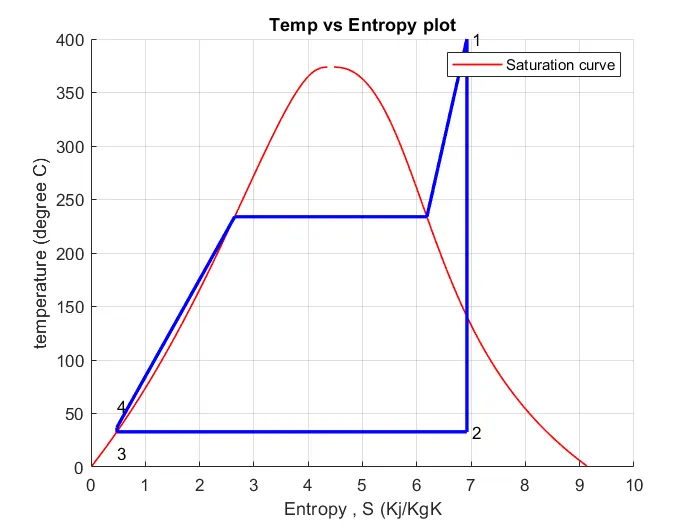
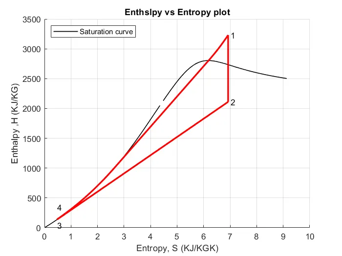
4. Plotting the T vs S and H vs S

Theory,

A Rankine cycle is an idealized thermodynamic cycle describing the process by which certain heat engines, such as steam turbines or reciprocating steam engines, allow mechanical work to be extracted from a fluid as it moves between a heat source and heat sink

Process ,

1. process 1-2 isentropic expansion in the turbine
2. process 2-3 constant pressure heat rejection in condensor
3. process 3-4 isentropic compression in the pump
4. process 4-1 constant pressure heat addition in the boiler

Rankine cycle efficiency

Efficiency = workdone/ Heat absorbed

= h2-h3/h2-hf3

Code for Rankine Cycle

clear all
close all
clc
disp(' RANKINE CYCLE');
disp('1-2 Constant pressure heat addition ithe boiler');
disp('2-3 isentropic Expansion in the turbine');
disp('3-4 Constant pressure heat removal in the condesor');
disp('4-1 Isentropic compression in the pump');

p1 = input('nValue of pressure at turbine inlet, p1(in bar) = ');
T1 = input('nvalue of temperture at tubine inlet, T1(in degree.C ) = ');
p2 = input('nValue of pressure at condesor inlet , p2(in bar) = ');

% At state 1
%extracting Enthalpy at state 1
h1 = XSteam('h_pT',p1,T1);
%similarly 
s1 = XSteam('s_pT', p1,T1);

%At state 2
s2 = s1;
sf2 = XSteam('sL_p', p2);
sg2 = XSteam('sV_p', p2);
x2 = (s2-sf2)/(sg2-sf2);
hf2 = XSteam('hL_p', p2);
hg2 = XSteam('hV_p', p2);
h2 = hf2+(x2*(hg2-hf2));

%At state 3
p3 = p2;
s3 = XSteam('sL_P', p3);
h3 = XSteam('hL_P', p3);

%At state 4
s4 = s3;
p4 = p1;

%Work done by turbine
Wt = h1 - h2 ;

% work done to run the pump
v3 = XSteam('vL_P', p3);
Wp = v3*(p4 - p3)*100;
h4 = h3 + Wp;

%Net work
Wnet= Wt - Wp;

%heat into the system
Qin = h1 - h4;

% Heat out of the system
Qout = h2 - h3;

%Thermal efficiency
thermal_eff = (Wnet/Qin)*100;

%specific steam consumption
%ssc = mass flow rate/ poer
SSC = (3600/Wnet);

%back work ratio
BW = (Wp/Wt);

% calculation of temperature at state points
T3 = XSteam('Tsat_p', p3);
T2 = T3;
Cp4 = XSteam('Cp_ps', p4, s4);
Cv4 = XSteam('Cv_ps', p4, s4);
k = Cp4/Cv4;
T4 = T3/((p3/p4)^((k-1)/k));

% calculatigTemperature, entropy and enthalpy at the vapour and liquid line for plotting
T6 = XSteam('Tsat_p', p1);
s5 = XSteam('sL_p', p1);
s6 = XSteam('sV_p', p1);
h5 = XSteam('hL_P', p1);
h6 = XSteam('hV_P', p1);
T5 = T6;

%plotting the saturation curve
T = linspace(1,375,1000);
for i = 1:length(T)
    sf(i) = XSteam('sL_T', T(i));
    sg(i) = XSteam('sV_T', T(i));
    hf(i) = XSteam('hL_T', T(i));
    hg(i) = XSteam('hV_T', T(i));
end

%plotting T-S diagram
figure(1)
hold on
plot(sf,T,'r','linewidth',1)
plot(sg,T,'r','linewidth',1)
plot([s1 s2], [T1 T2], 'b', 'LineWidth',2)
plot([s2 s3], [T2 T3], 'b', 'LineWidth',2)
plot([s3 s4], [T3 T4], 'b', 'LineWidth',2)
plot([s4 s5], [T4 T5], 'b', 'LineWidth',2)
plot([s5 s6], [T5 T6], 'b', 'LineWidth',2)
plot([s6 s1], [T6 T1], 'b', 'LineWidth',2)
sc1 = linspace(s6,s1,1000);
for l = 1:length(sc1)
    Tc1(l)= XSteam('T_ps',p1,sc1(1));
end

text(s1+0.1, T1, '1')
text(s2+0.1,T2,'2')
text(s3, T3-20, '3')
text(s4, T4+20,'4')
title('Temp vs Entropy plot')
xlabel('Entropy , S (Kj/KgK')
ylabel('temperature (degree C)')
legend('Saturation curve')
grid on
%Plotting h-s Diagram
figure(2)
hold on
grid on
plot(sf,hf,'k','linewidth',1)
plot(sg,hg,'k', 'linewidth',1)
plot([s1 s2], [h1 h2],'r','linewidth',2)
plot([s2 s3], [h2 h3],'r','linewidth',2)
plot([s3 s4], [h3 h4],'r','linewidth',2)
hc = linspace(h4, h1, 100);
for r = 1:length(hc)
    sch(r) = XSteam('s_ph',p1,hc(r));
end
plot(sch,hc, 'r','linewidth',2)

for m = 1:length(sc1)
    hc1(m) = XSteam('h_ps',p1,sc1(m));
end
plot(sc1,hc1, 'r','linewidth',2)
text(s1+0.1,h1,'1')
text(s2+0.1,h2,'2')
text(s3, h3-100,'3')
text(s4, h4+200,'4')
title('Enthslpy vs Entropy plot')
xlabel('Entropy, S (KJ/KGK)')
ylabel('Enthalpy ,H (KJ/KG)')
legend('Saturation curve','location','northwest')

% displaying the results in the command window
disp('Results');
p1 = p1;
T1 = T1;
p2 = p2;
disp('At stage point 1');
n1 = sprintf('P1 is %.3f bar',p1);
disp(n1);
n2 = sprintf('T1 is %.3f c',T1);
disp(n2);
n3 = sprintf('h1 is %.3f kj/kg',h1);
disp(n3);
n4 = sprintf('s1 is %.3f kj/kgk',s1);
disp(n4);
disp('At stage point 2');
n11 = sprintf('P2 is %.3f bar',p2);
disp(n11);
n21 = sprintf('T2 is %.3f c',T2);
disp(n21);
n31 = sprintf('h2 is %.3f kj/kg',h2);
disp(n31);
n41 = sprintf('s2 is %.3f kj/kgk',s2);
disp(n41);
disp('At stage point 3')
n12 = sprintf('P3 is %.3f bar',p3);
disp(n12);
n22 = sprintf('T3 is %.3f c',T3);
disp(n22);
n32 = sprintf('h3 is %.3f kj/kg',h3);
disp(n32);
n42 = sprintf('s3 is %.3f kj/kgk',s3);
disp(n42);
disp('At stage point 4')
n13 = sprintf('P4 is %.3f bar',p4);
disp(n13);
n23 = sprintf('T4 is %.3f c',T4);
disp(n23);
n33 = sprintf('h4 is %.3f kj/kg',h4);
disp(n33);
n43 = sprintf('s4 is %.3f kj/kgk',s4);
disp(n43);
n14 = sprintf('Wt is %.3f kj/kg',Wt);
disp(n14);
n15 = sprintf('Wp is %.3f kg/kj',Wp);
disp(n15);
n16 = sprintf('Wnet is %.3f kj/kg',Wnet);
disp(n16);
n17 = sprintf('Thermal_efficiency is %.2f percent',thermal_eff);
disp(n17);
n18 = sprintf('SSC is %.2f',SSC);
disp(n18);
n19 = sprintf('Back work ratio is %.3f ',BW);
disp(n19);

Results

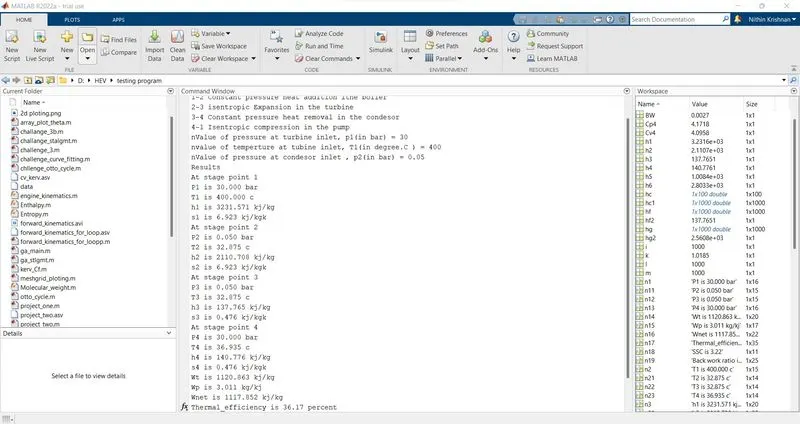
1.Network Done = 1120.863 Kj/Kg

2.Thermal Efficiency = 36.17%

3.Back Work ratio= 0.003