Week 3 - Taylor table method and Matlab code

Objective: Evaluate the second order derivative of the given analytical function using 4th order approximation techniques (central difference, skewed right-sided difference, skewed right-sided difference) and compare the absolute error between them.

Analytical function: `f(x) = exp(x)*cos(x)`

fourth order approximations:

• Central difference

  	`f(i)`	`trianglex^2 f'(x)`	`trianglex^3 f''(x)`	`trianglex^4 f'''(x)`	`trianglex^5 f^4(x)`
  `af(i-2)`	a	-2a	`(4a)/2`	`-(8a)/6`	`(16e)/24`
  `bf(i-1)`	b	-b	`b/2`	`-(b)/6`	`b/24`
  `cf(i)`	c	0	0	0	0
  `df(i+1)`	d	d	`d/2`	`d/6`	`d/24`
  `ef(i+2)`	e	2e	`(4e)/2`	`(8e)/6`	`(16e)/24`
  	`Sigma`= 0	`Sigma`= 0	`Sigma`= 1	`Sigma`= 0	`Sigma`= 0

• The order of accuracy (P) = Number of nodes in the stencil (N) - order of derivative (Q) + 1
• P = 5 - 2 + 1 = 4

hence the scheme is fourth order accurate.

• Skewed right-sided difference

  	`f(i)`	`trianglexf'(i)`	`trianglex^2f''(i)`	`trianglex^3f'''(i)`	`trianglex^4f^4(i)`	`trianglex^5f^5(i)`
  `af(i)`	a	0	0	0	0	0
  `bf(i+1)`	b	b	`b/2`	`b/6`	`b/24`	`b/120`
  `cf(i+2)`	c	2c	`(4c)/2`	`(8c)/6`	`(16c)/24`	`(32c)/120`
  `df(i+3)`	d	3d	`(9d)/2`	`(27d)/6`	`(81d)/24`	`(243d)/120`
  `ef(i+4)`	e	4e	`(16e)/2`	`(64e/6)`	`(256e)/24`	`(1024e)/120`
  `gf(i+5)`	g	5g	`(25g)/2`	`(125g)/6`	`(625g)/24`	`(3125g)/120`
  	`Sigma`= 0	`Sigma`= 0	`Sigma`= 1	`Sigma`= 0	`Sigma`= 0	`Sigma`= 0

The order of accuracy (P) = Number of nodes in the stencil (N) - order of derivative (Q)

P = 6 - 2 = 4

Hence the scheme is fourth order accurate.

• Skewed left-sided difference

  	`f(i)`	`trianglexf'(i)`	`trianglex^2f''(i)`	`trianglex^3f'''(i)`	`trianglex^4f^4(i)`	`trianglex^5f^5(i)`
  `af(i-5)`	a	-5a	`(25a)/2`	`-(125a)/6`	`(625a)/24`	`-(3125a)/120`
  `bf(i-4)`	b	-4b	`(16b)/2`	`-(64b)/6`	`(256b)/24`	`-(1024b)/120`
  `cf(i-3)`	c	-3c	`(9c)/2`	`-(27c)/6`	`(81c)/24`	`-(243c)/120`
  `df(i-2)`	d	-2d	`(4d)/2`	`-(8d)/6`	`(16d)/24`	`-(32d)/120`
  `ef(i-1)`	e	-e	`e/2`	`-e/6`	`e/24`	`-e/120`
  `gf(i)`	g	0	0	0	0	0
  	`Sigma`= 0	`Sigma`= 0	`Sigma`= 1	`Sigma`= 0	`Sigma`= 0	`Sigma`= 0

The order of accuracy (P) = Number of nodes in the stencil (N) - order of derivative (Q)

P = 6 - 2 = 4

Hence the scheme is fourth order accurate.

Functions:

analytical function given in question.

function out = fun(z)
    out = exp(z)*cos(z);
end

central approximation function

function out = central_approx(x,dx,Xc,analytical_sol)
    
    % central-diffrence
    a = Xc(1); b = Xc(2); c = Xc(3); d = Xc(4); e = Xc(5);
    cd = (a*fun(x - 2*dx) + b*fun(x - dx) + c*fun(x) + d*fun(x + dx) + e*fun(x + 2*dx))/(dx^2);
    out = abs(cd - analytical_sol); % Absolute error.
    
end

skewed right-sided difference function

function out = xrd_approx(x,dx,Xr,analytical_sol)
    
    % Skewed right-sided difference
    a = Xr(1); b = Xr(2); c = Xr(3); d = Xr(4); e = Xr(5); g = Xr(6);
    srd = (a*fun(x) + b*fun(x + dx) + c*fun(x + 2*dx) + d*fun(x + 3*dx) + e*fun(x + 4*dx) + g*fun(x + 5*dx))/(dx^2);
    error_srd = abs(srd - analytical_sol); % Absolute error. 
    out = error_srd;

end

Skewed left-sided difference function

function out = xld_approx(x,dx,Xl,analytical_sol)
    
    % Skewed left-sided difference
    a = Xl(1); b = Xl(2); c = Xl(3); d = Xl(4); e = Xl(5); g = Xl(6);
    sld = (a*fun(x - 5*dx) + b*fun(x - 4*dx) + c*fun(x - 3*dx) + d*fun(x - 2*dx) + e*fun(x - dx) + g*fun(x))/(dx^2);
    error_sld = abs(sld - analytical_sol); % Absolute error.
    out = error_sld;
end

Matlab Program:

clear all; close all; clc;
% Program compares the 
x = pi/3; % Initialization.
dx = linspace(pi/30,pi/300,40); % Defining Grid Spacing.

    % coefficints for central approximation.
    syms a b c d e
    eqn1 = a + b + c + d + e == 0;
    eqn2 = -2*a - b + d + 2*e == 0;
    eqn3 = (4/2)*a + (1/2)*b + (1/2)*d + (4/2)*e == 1;
    eqn4 = -(8/6)*a - (1/6)*b + (1/6)*d + (8/6)*e == 0;
    eqn5 = (16/24)*a + (1/24)*b + (1/24)*d + (16/24)*e == 0;

    [A,B] = equationsToMatrix([eqn1, eqn2, eqn3, eqn4, eqn5],[a, b, c, d, e]);

    Xc = linsolve(A,B);
    % Coefficients for skewed right-sided difference.
    clear a b c d e eqn1 eqn2 eqn3 eqn4 eqn5
    syms a b c d e g
    eqn1 = a + b + c + d + e + g == 0;
    eqn2 = b + 2*c + 3*d + 4*e + 5*g == 0;
    eqn3 = (1/2)*b + (4/2)*c + (9/2)*d + (16/2)*e + (25/2)*g == 1;
    eqn4 = (1/6)*b + (8/6)*c + (27/6)*d + (64/6)*e + (125/6)*g == 0;
    eqn5 = (1/24)*b + (16/24)*c + (81/24)*d + (256/24)*e + (625/24)*g == 0;
    eqn6 = (1/120)*b + (32/120)*c + (243/120)*d + (1024/120)*e + (3125/120)*g == 0;

    [A,B] = equationsToMatrix([eqn1, eqn2, eqn3, eqn4, eqn5, eqn6],[a, b, c, d, e, g]); 

    Xr = linsolve(A,B);
    % Coefficients for skewed left-sided difference.
    clear a b c d e g eqn1 eqn2 eqn3 eqn4 eqn5 eqn6
    syms a b c d e g
    eqn1 = a + b + c + d + e + g == 0;
    eqn2 = -5*a - 4*b - 3*c - 2*d - e == 0;
    eqn3 = (25/2)*a + (16/2)*b + (9/2)*c + (4/2)*d + (1/2)*e == 1;
    eqn4 = -(125/6)*a - (64/6)*b - (27/6)*c - (8/6)*d - (1/6)*e == 0;
    eqn5 = (625/24)*a + (256/24)*b + (81/24)*c + (16/24)*d + (1/24)*e == 0;
    eqn6 = -(3125/120)*a - (1024/120)*b - (243/120)*c - (32/120)*d - (1/120)*e == 0;

    [A,B] = equationsToMatrix([eqn1, eqn2, eqn3, eqn4, eqn5, eqn6],[a, b, c, d, e, g]);

    Xl = linsolve(A,B);
    
% analytical solution
analytical_sol = - 2*exp(x)*sin(x);

% calculating the errors
for i = 1:length(dx)
   % Absolute errors.
   central_error(i) = central_approx(x,dx(i),Xc,analytical_sol);
   
   xrd_error(i) = xrd_approx(x,dx(i),Xr,analytical_sol);
    
   xld_error(i) = xld_approx(x,dx(i),Xl,analytical_sol);
    
end

% Plotting the figure.
figure % Defining figure window.
% plotting log plot for better visuatization and comparison.
loglog(dx,central_error,'b--d')
hold on
loglog(dx,xrd_error,'r--s')
hold on
loglog(dx,xld_error,'g--o')

title('Comparision of numerical approximation methods in the range of dx')
xlabel('Spacing between two nodes (dx)') %specifying x label.
ylabel('Absolute Error') % specifying y label.
legend('Central difference','Skew right-sided difference','Skew left-sided difference') % specifying label to the curves.

Results and conclusion:

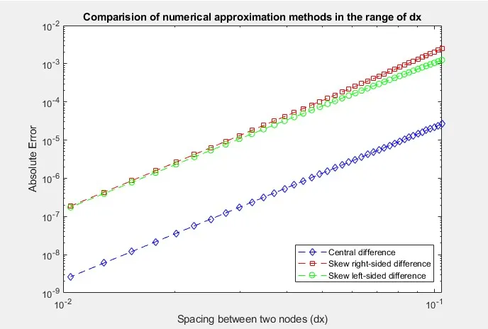
As it can be observed from the output figure that the central difference scheme have least error then the other two schemes. and lower the grid size (dx), lower will be the error.

but reducing the grid size to get less error will work till a certain point after that if grid size reduced further the error will increase significantly instead of reducing further. as we can observe from the blow graph.

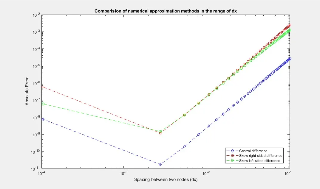
Even if central diff scheme produced significanty lower absolute error. the skewed schemes are still required because CD scheme require values in both left and right node, which may not present is all cases. In those cases skewed schemes are useful and can be use without losing the fourth order accuracy.