Week 3 - Taylor table method and Matlab code

Problem statement:-

Deriving a fourth order approximation of second order derivative using three different schemes like central difference, Skewed right side and skewed left side through taylor table method.

Comparing the second order derivative of analytical function with three numerical approximation.

Introduction:-

Taylor table is a method which is used to derive expression for second order derivative of a function to obtain different numerical scheme in order to meet desired accuracy.

Different numerical schemes like Central difference, skewed right sided difference, skewed left sided difference are used to obtain fourth order approximation of second derivative.

Numerical discretization transfers the continuous function into discrete points. Number of nodes are decided by the given equation:-

`n = p + q`

where n= number of nodes

p= order of derivative

q= order of approximation

Therefore, for skewed scheme number of derivative is equal to 6

In central difference scheme, number of nodes are decided by

`n = p + q - 1`

Derivation:-

1:- Central Difference:-

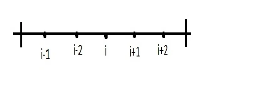
To develop fourth order accurate approximation to second order derivative at node i which involves nodes i-2, i-1,i and subsequent nodes to the right of i. `f_i^(2)` requires 5 nodes for `O(Deltax)^4` accuracy.

Therefore, we consider nodes :-

`frac{del^2f}{del x^2}` is approximated as:-

`frac{del^2f}{delx^2} ~~ f^{''} -`Error = `frac{af(i-2)+bf(i-1)+cf(i)+df(i+1)+ef(i+2)}{Deltax^2}`

above equation can be written as:-

`f^(2)-Deltax^4 f^(6)`(constant)=`frac{af(i-2)+bf(i-1)+cf(i)+df(i+1)+ef(i+2)}{Deltax^2}`

Therefore in error term, the power of `Delta x` is 4. This shows that central difference is 4th order appproximation.

Taylor's table for fourth order approximation of second order derivative using central difference:-

NUMERICAL STENCIL	TAYLOR’S TABLE TERMS
		f(i)	(∆x)f1(i)	(∆x)2f2(i)	(∆x)3f3(i)	(∆x)4f4(i)	(∆x)5f5(i)
	af(i-2)	a	(-2a)	(4a)/2	(-8a)/6	(16a)/24	(-32a)/120
	bf(i-1)	b	(-b)	(b)/2	(-b)/6	(b)/24	(-b)/120
	cf(i)	c	0	0	0	0	0
	df(i+1)	d	d	d/2	d/6	d/24	d/120
	ef(i+2)	e	2e	4e/2	8e/6	16e/24	32e/120
Coefficients in Equation		0	0	1	0	0	0

Equation is solved through matlab is given below:

clc;
clear all;
close all;

A= [1 1 1 1 1; -2 -1 0 1 2; 4/2 1/2 0 1/2 4/2; -8/6 -1/6 0 1/6 8/6; 16/24 1/24 0 1/24 16/24; -32/120 -1/120 0 1/120 32/120];

B=[0;0;1;0;0;0]
c=(linsolve(A,B))

The output is:-

c =

   -0.0833
    1.3333
   -2.5000
    1.3333
   -0.0833

the equation is:-

`frac{del^2 f}{del x^2}~~frac{ -0.0833f(i-2)+1.3333f(i-1)-2.500f(i)+1.3333f(i+1)-0.0833f(i+2)}{Delta x^2}`

2:- Skewed right-sided difference:-

In this, to develop fourth order approximation to second order derivative at node i which involves subsequent node to the right side of i like i+1,i+2,i+3,i+4...so on. This scheme requires 6 nodes for `O(Delta x^4)`accuracy.

Therefore, we consider the nodes like:-

`frac{del^2 f}{delx^2}~~f^2(x )-Deltax^4 f^6(x)`(constant) =`frac{af(i)+bf(i+1)+cf(i+2)+df(i+3)+ef(i+4)+gf(i+5)}{Deltax^2}`

Therefore, Error term `Deltax^4 f^6(x)` which of the order 4.

This shows that the skewed right sided difference is fourth order accurate.

Taylor's Table for fourth order approximation of second derivative :-

NUMERICAL STENCIL	TAYLOR’S TABLE TERMS
		f(i)	(∆x)f1(i)	(∆x)2f2(i)	(∆x)3f3(i)	(∆x)4f4(i)	(∆x)5f5(i)
	af(i)	a	0	0	0	0	0
	bf(i+1)	b	b	b/2	b/6	b/24	b/120
	cf(i+2)	c	2c	4c/2	8c/6	16c/24	32c/120
	df(i+3)	d	3d	9d/2	27d/6	81d/24	243d/120
	ef(i+4)	e	4e	16e/2	64e/6	256e/24	1024e/120
	gf(i+5)	g	5g	25g/2	125g/6	625g/24	3125g/120
Coefficients in Equation		0	0	1	0	0	0

Equation is solved by matlab is given by:-

clc;
clear all;
close all;

A= [1 1 1 1 1 1; 0 1 2 3 4 5;0 1/2 4/2 9/2 16/2 25/2; 0 1/6 8/6 27/6 64/6 125/6 ; 0 1/24 16/24 81/24 256/24 625/24;
   0 1/120 32/120 243/120 1024/120 3125/120];

B=[0;0;1;0;0;0]
c=(linsolve(A,B))

The output is:-

c =

    3.7500
  -12.8333
   17.8333
  -13.0000
    5.0833
   -0.8333

`frac{del^2f}{delx^2}~~frac{3.75f(i)-12.8333f(i+1)+17.8333f(i+2)-13f(i+3)+5.0833f(i+4)-0.08333f(i+5)}{Delta x^2}`

3:- Skewed left-sided difference:-

In this, to develop fourth order approximation to second order derivative at node i which involves subsequent node to the left side of i like i-1,i-2,i-3,i-4...so on. This scheme requires 6 nodes for `O(Delta x^4)`accuracy.

Therefore, we consider the nodes like:-

`frac{del^2f}{delx^2}~~frac{af(i-5)+bf(i-4)+cf(i-3)+df(i-2)+ef(i-1)+gf(i)}{Delta x^2}`

Therefore, Error term `Deltax^4 f^6(x)` which of the order 4.

This shows that the skewed left sided difference is fourth order accurate.

Taylor's Table for fourth order approximation of second derivative :-

NUMERICAL STENCIL	TAYLOR’S TABLE TERMS
		f(i)	(∆x)f1(i)	(∆x)2f2(i)	(∆x)3f3(i)	(∆x)4f4(i)	(∆x)5f5(i)
	af(i-5)	a	-5a	25a/2	-125a/6	625a/24	-3125a/120
	bf(i-4)	b	-4b	16b/2	-64b/6	256b/24	-1024b/120
	cf(i-3)	c	-3c	9c/2	-27c/6	81c/24	-243c/120
	df(i-2)	d	-2d	4d/2	-8d/6	16d/24	-32d/120
	ef(i-1)	e	-e	e/2	-e/6	e/24	-e/120
	gf(i)	g	0	0	0	0	0
Coefficients in Equation		0	0	1	0	0	0

Equation is solved by matlab is given below:-

clc;
clear all;
close all;

A= [1 1 1 1 1 1;-5 -4 -3 -2 -1 0; 25/2 16/2 9/2 4/2 1/2 0; -125/6 -64/6 -27/6 -8/6 -1/6 0 ;625/24 256/24 81/24 16/24 1/24 0;
   -3125/120 -1024/120 -243/120 -32/120 -1/120 0];

B=[0;0;1;0;0;0]
c=(linsolve(A,B))

The output is :-

c =

   -0.8333
    5.0833
  -13.0000
   17.8333
  -12.8333
    3.7500

`frac{del^2 f}{delx^2}~~ frac{-0.8333f(i-5)+5.0833f(i-4)-13f(i-3)+17.8333f(i-2)-12.8333f(i-1)+3.7500f(i)}{Delta x^2}`

MATLAB CODE:-

A:-

clear all;
close all;
clc; 
x=pi/3;
dx=linspace(pi/4,pi/400,20)
%exact derivative
analy=(-2)*exp(x)*sin(x);
for i=1:length(dx)
central_diff(i)=(-1*fun(x-2*dx(i))+16*fun(x-dx(i))-30*fun(x)+16*fun(x+dx(i))-1*fun(x+2*dx(i)))/(12*(dx(i)^2));
%Skewed right-sided difference scheme
skewed_right(i)=(45*fun(x)-154*fun(x+dx(i))+214*fun(x+2*dx(i))-156*fun(x+3*dx(i))+61*fun(x+4*dx(i))-10*fun(x+5*dx(i)))/(12*(dx(i)^2));
%Skewed left-sided difference scheme
skewed_left(i)=(45*fun(x)-154*fun(x-dx(i))+214*fun(x-2*dx(i))-156*fun(x-3*dx(i))+61*fun(x-4*dx(i))-10*fun(x-5*dx(i)))/(12*dx(i)^2);
end
%computing error

central_err=abs(analy-central_diff);
skewed_right_err=abs(analy-skewed_right);
skewed_left_err=abs(analy-skewed_left);
loglog(dx,central_err,'-*r');
%plot(dx,central_err,'-*r');
hold on;
loglog(dx,skewed_right_err,'-dk');
%plot(dx,skewed_right_err,'-dk');
hold on;
loglog(dx,skewed_left_err,'-og');
%plot(dx,skewed_left_err,'-og');
grid on;
ylabel('Absolute Error');
xlabel('dx');
legend('Central difference ','Skewed right-sided ','Skewed left-sided','location','best');

B:-Function files:-

function out = fun(x)
out =exp(x)*cos(x);
end

Output:-

For range of dx=linspace(pi/4,pi/400,20)

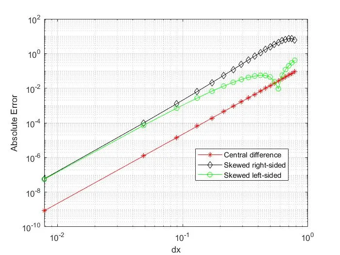
The above plot is loglog plot between absolute error of different scheme vs dx. In this plot as dx is increasing, absolute error is increasing. Absolute error is less for central difference as compared to skewed schemes. In central difference, absolute error is starting from 10^-9 , point lower than skewed scheme which starts from 10^(-7).As we can see both skewed scheme gives same error upto 10^(-4). After 10^(-4), slope of absolute error of skewed right-sided is greater than skewed left-sided. Central difference , skewed right-side has constant slope While slope of skewed left sided is keep on decreasing upto at some value of dx after that it is increasing.

For range of dx=linspace(pi/4,pi/40000,20)

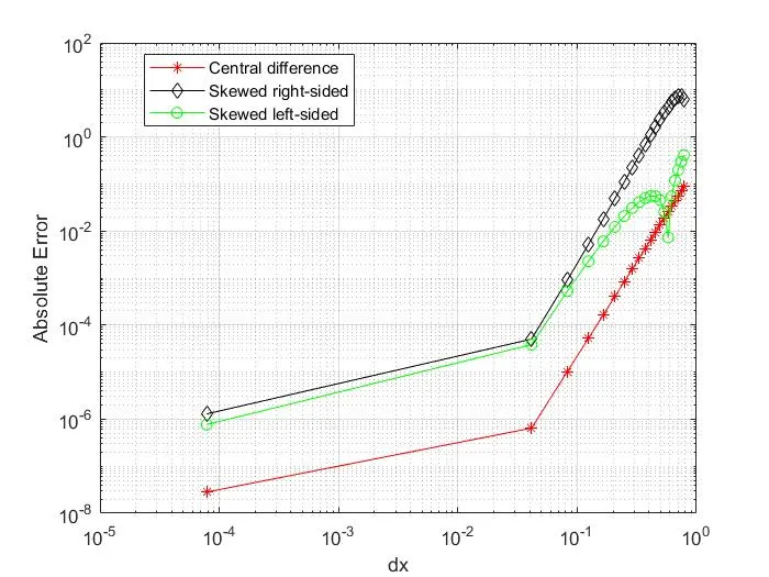
Central difference approximation has smaller error for small values of dx. As value of dx increases error is also increasing. We further extend the value of dx slope of scheme increases.Change in slope shows the inability of the machine to represent it accurately as the number becomes smaller smaller.

Therefore, it shows that central difference gives more accurate result and other two.But skewed scheme is prefered over central difference because central difference scheme is not applied at the boundary node as we need information about right and left nodes at the same time.

Conclusion:-

1:-Central difference scheme has smaller error as compared to both skewed schemes.

central difference error < Skewed left-sided error `~<` skewed right sided.

2:- Skewed schemes are prefered over central due to unavailability of left and right nodes about boundary node