Taylor table method and Matlab code - a comparison of Central Difference,Right Skewed and Left Skewed Methods
Central Difference
Number of nodes for central difference method = p + q -1
= 2 + 4 -1 = 5
`(trianglex)^2*(d^2y)/(dx^2)` = a*f(i-2) + b*f(i-1) + c*f(i) + d*f(i+1) + e*f(i+2)
Taylor Table
| f(i) | `(trianglex)f'(i)` | `(trianglex)^2f^2(i)` | `(trianglex)^3f^3(i)` | `(trianglex)^4f^4(i)` | `(trianglex)^5f^5(i)` | `(trianglex)^6f^6(i)` | |
| a*f(i-2) | a | -2a | 2a | -8a/6 | 16a/24 | -32a/120 | 64a/720 |
| b*f(i-1) | b | -b | b/2 | -b/6 | b/24 | -b/120 | b/720 |
| c*f(i) | c | 0 | 0 | 0 | 0 | 0 | 0 |
| d*f(i+1) | d | d | d/2 | d/6 | d/24 | d/120 | d/720 |
| e*f(i+2) | e | 2e | 2e | 8e/6 | 16e/24 | 32e/120 | 64e/720 |
| 0 | 0 | 1 | 0 | 0 |
Considering the coefficients above, a system of linear equations are formed as below
a + b + c + d + e = 0
-2a - b + 0 + d + 2e = 0
2a + b/2 + 0 + d/2 + 2e = 1
-8a/6 - b/6 + 0 + d/6 + 8e/6 = 0
16a/24 + b/24 + 0 + d/24 + 16e/24 = 0
Matlab code inorder to solve the above set of equations
Solving the above equations, we get
a = -1/12
b = 4/3
c = -5/2
d = 4/3
e = -1/12
Hence, the fourth order approximate can be expressed as
`(d^2y)/(dx^2) = (-f(i-2) + 16f(i-1) - 30f(i) + 16f(i+1) - f(i+2))/(12(trianglex)^2)`
Skewed Right sided
Number of nodes = p + q = 2 + 4 = 6
`(trianglex)^2*(d^2y)/(dx^2)` = a*f(i) + b*f(i+1) + c*f(i+2) + d*f(i+3) + e*f(i+4) + g*f(i+5)`
| f(i) | `(trianglex)f'(i)` | `(trianglex)^2f^2(i)` | `(trianglex)^3f^3(i)` | `(trianglex)^4f^4(i)` | `(trianglex)^5f^5(i)` | `(trianglex)^6f^6(i)` | |
| a*f(i) | a | 0 | 0 | 0 | 0 | 0 | 0 |
| b*f(i+1) | b | b | b/2 | b/6 | b/24 | b/120 | b/720 |
| c*f(i+2) | c | 2c | 2c | 8c/6 | 16c/24 | 32c/120 | 64c/720 |
| d*f(i+3) | d | 3d | 9d/2 | 27d/6 | 81d/24 | 243d/120 | 729d/720 |
| e*f(i+4) | e | 4e | 8e | 64e/6 | 256e/24 | 1024e/120 | 4096e/720 |
| g*f(i+5) | g | 5g | 25g/2 | 125g/6 | 625g/24 | 3125g/120 | 15625g/720 |
| 0 | 0 | 1 | 0 | 0 | 0 |
Considering the coefficients above, a system of linear equations are formed as below
a + b + c + d + e + g = 0
0 + b + 2c + 3 d + 4e + 5g = 0
0 + b/2 + 2c + 9d/2 + 8e + 25g/2 = 1
0 + b/6 + 8c/6 + 27d/6 + 64e/6 +125g/6 = 0
0 + b/24 + 16c/24 + 81d/24 + 256e/24 + 625g/24 = 0
0 + b/120 + 32c/120 + 243d/120 + 1024e/120 + 3125g/120 = 0
Matlab code inorder to solve the above set of equations
Solving the above equations, we get
a = 15/4
b = -77/6
c = 107/6
d = -13
e = 61/12
g = -5/6
`(d^2y)/(dx^2) = (45f(i) - 154f(i+1) + 214f(i+2) - 156f(i+3) + 61f(i+4) - 10f(i+5))/(12(trianglex)^2)`
Skewed left sided
Number of nodes = p + q = 2 + 4 = 6
`(trianglex)^2*(d^2y)/(dx^2)` = a*f(i) + b*f(i-1) + c*f(i-2) + d*f(i-3) + e*f(i-4) + g*f(i-5)`
| f(i) | `(trianglex)f'(i)` | `(trianglex)^2f^2(i)` | `(trianglex)^3f^3(i)` | `(trianglex)^4f^4(i)` | `(trianglex)^5f^5(i)` | `(trianglex)^6f^6(i)` | |
| a*f(i) | a | 0 | 0 | 0 | 0 | 0 | 0 |
| b*f(i-1) | b | -b | b/2 | -b/6 | b/24 | -b/120 | b/720 |
| c*f(i-2) | c | -2c | 2c | -8c/6 | 16c/24 | -32c/120 | 64c/720 |
| d*f(i-3) | d | -3d | 9d/2 | -27d/6 | 81d/24 | -243d/120 | 729d/720 |
| e*f(i-4) | e | -4e | 8e | -64e/6 | 256e/24 | -1024e/120 | 4096e/720 |
| g*f(i-5) | g | -5g | 25g/2 | -125g/6 | 625g/24 | -3125g/120 | 15625g/720 |
| 0 | 0 | 1 | 0 | 0 | 0 |
Considering the coefficients above, a system of linear equations are formed as below
a + b + c + d + e + g = 0
0 - b - 2c - 3 d - 4e - 5g = 0
0 + b/2 + 2c + 9d/2 + 8e + 25g/2 = 1
0 - b/6 - 8c/6 - 27d/6 - 64e/6 - 125g/6 = 0
0 + b/24 + 16c/24 + 81d/24 + 256e/24 + 625g/24 = 0
0 - b/120 - 32c/120 - 243d/120 - 1024e/120 - 3125g/120 = 0
Matlab code inorder to solve the above set of equations
Solving the above equations, we get
a = 15/4
b = -77/6
c = 107/6
d = -13
e = 61/12
g = -5/6
`(d^2y)/(dx^2) = (45f(i) - 154f(i-1) + 214f(i-2) - 156f(i-3) + 61f(i-4) - 10f(i-5))/(12(trianglex)^2)`
Matlab Program
% function file for mathematical expression
function math = func(x)
    math = exp(x)*cos(x); %function
end
% function file to calculate error by central difference method
function out = central_diff(x,dx)

     analytical_value = -2*exp(x)*sin(x);   %second derivative of the function

     %function calling for numerical value calculation
     a = func(x-2*dx)/(12*(dx)^2);
     b = func(x-dx)/(12*(dx)^2);
     c = func(x)/(12*(dx)^2);
     d = func(x+dx)/(12*(dx)^2);
     e = func(x+2*dx)/(12*(dx)^2);

     numerical_value = -a+16*b-30*c+16*d-e;
     out = abs(analytical_value-numerical_value); %absolute error
end
% function file to calculate error using Skewed right sided difference method
function out = right_skew(x,dx)

    analytical_value = -2*exp(x)*sin(x); %second derivative of the function

    % function calling for numerical value calculation
    a = func(x)/(12*(dx)^2);
    b = func(x+dx)/(12*(dx)^2);
    c = func(x+2*dx)/(12*(dx)^2);
    d = func(x+3*dx)/(12*(dx)^2);
    e = func(x+4*dx)/(12*(dx)^2);
    f = func(x+5*dx)/(12*(dx)^2);

   numerical_value = 45*a-154*b+214*c-156*d+61*e-10*f;

   out = abs(analytical_value-numerical_value); % absolute error

end
% function file to calculate error using skewed left sided difference method
function out = left_skew(x,dx)

    analytical_value = -2*exp(x)*sin(x);  % second derivative of the function

    %function calling for numerical value calculation
    a = func(x)/(12*(dx)^2);
    b = func(x-dx)/(12*(dx)^2);
    c = func(x-2*dx)/(12*(dx)^2);
    d = func(x-3*dx)/(12*(dx)^2);
    e = func(x-4*dx)/(12*(dx)^2);
    f = func(x-5*dx)/(12*(dx)^2);

   numerical_value = 45*a-154*b+214*c-156*d+61*e-10*f;

   out = abs(analytical_value-numerical_value);   %absolute error
end
% Matlab script file
close all
clc

x = pi/3; % value of x
dx = linspace(pi/4,pi/300,100); % range of values of dx


% function call for error calculation
for i = 1:length(dx)
    central_diff_error(i) = central_diff(x,dx(i));
    right_skew_error(i) = right_skew(x,dx(i));
    left_skew_error(i) = left_skew(x,dx(i));
end

% graph plotting
figure(1);
xlabel('dx')
ylabel('Absolute Error')
loglog(dx,central_diff_error,'r')
hold on;
loglog(dx,right_skew_error,'g')
hold on;
loglog(dx,left_skew_error,'b')
legend('Central Difference','Skewed Right Sided Difference','Skewed Left Sided Difference')
Output
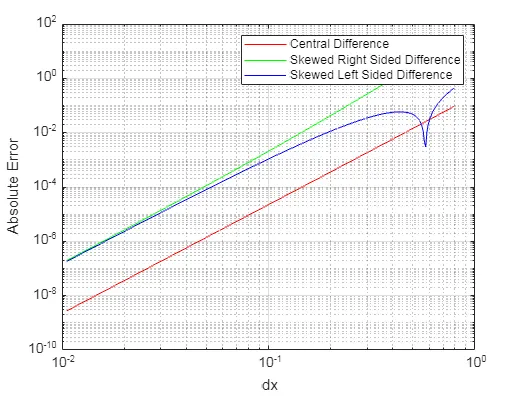
Graph - Absolute Error Vs dx
Result
1) Central Difference method is having the very low error of order (10^-8) for very small values of dx,(0.01<dx<0.1). Hence it gives the most accurate result.
2) For relatively high values of dx,(0.2<dx<1), Skewed left sided method gives better result than central difference method since it has the lowest error.
3) For very small values of dx, skewed right sided difference and skewed left sided difference gives almost same values of absolute error.