Week 3 - Taylor table method and Matlab code

In this project, we have to derive the fourth order approximations for the second order derivative with central difference, skewed right sided difference, and skewed left sided difference schemes . The same has to be applied to a given second order derivative function exp(x)*cos(x). The Taylor Table method is used for the above said problem.

Taylor Table method for Central Difference Scheme:

Consider a numerical stencil such as

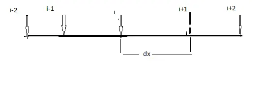
∂²u/∂x²»af(i-2)+bf(i-1)+cf(i)+df(i+1)+ef(i+2)

representing it as a linear algebraic system of equations, we get

a+b+c+d+e=0

-2a-b+0+d+2e=0

2a+b/2+0+d/2+2e=1

-8a/6-b/6+0+d/6+8e/6=0

16a/24+b/24+0+d/24+16e/24=0

solving the above equation using matlab and we get the values of a=-0.08333;b=1.33333;c=-2.50000;d=1.33333;e=-0.08333.

Substituting the value sof a,b,c,d e in the central difference equation of second order derivative, we get

∂²u/∂x²=-0.08333f(i-2)+1.33333f(i-1)-2.50000f(i)+1.33333f(i+1)-0.08333f(i+2)

Taylor Table method for Right Skewed Scheme

Consider a numerical stencil

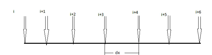
∂²u/∂x²=af(i)+bf(i+1)+cf(i+2)+df(i+3)+ef(i+4)+gf(i+5)

	f(i)	Δx.fI(i)	Δx^2.fII(i)	Δx^3.fIII(i)	Δx^4fIѵ(i)	Δx^5fѵ(i)	Δx^6fѵi(i)
af(i)	a	0	0	0	0	0	0
bf(i+1)	b	b	b/2	b/6	b/24	b/120	b/720
cf(i+2)	c	2c	4/2c	4/2c	16/24c	32c/120	64/720c
df(i+3)	d	3d	9/2d	9/2d	81/24d	243d/120	729/720d
ef(i+4)	e	4c	16/2e	64/6e	256/24e	1024e/120	4096/720e
gf(i+5)	g	5g	25/2g	125/6g	625/24g	3125g/120	15625/720g
sum	0	0	1	0	0	0	0

The system of linear algebraic equation of the above table

a+b+c+d+e=0

0+b+2c+3d+4e+5g=0

0+b/2+4c/2+9d/2+16e/2+25g/2=1

0+b/6+8c/6+27d/6+64e/6+125/6g=0

0+b/24+16c/24+81d/24+256e/24+625/24g=0

0+b/120+2^5/120c+3^5/120d+4^5/120e+5^5/120g=0

solving the above algebraic system of linear equations using matlab, we get

a=3.75000;b=-12.83333;c=17.83333;d=-13.00000;e=5.08333;g=-0.83333

substituting the values of coefficients in the right skewed difference equation we get

∂²u/∂x²=3.75000*f(i)-12.83333*f(i+1)+17.8333*f(i+2)-13.00000*f(i+3)+5.08333*f(i+4)-0.83333*f(i+5)

Taylor Table Method for Left Skewed Scheme

consider a numerical stencil for the scheme

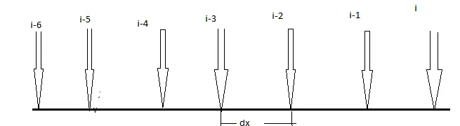
∂²u/∂x²=a*f(i)+b*f(i-1)+c*f(i-2)+d*f(i-3)+e*f(i-4)+g*f(i-5)

	f(i)	Δx.fI(i)	Δx^2.fII(i)	Δx^3.fIII(i)	Δx^4fIѵ(i)	Δx^5fѵ(i)	Δx^6fѵi(i)
af(i-5)	a	-5a	25/2a	-125/6a	625/24a	-3125a/120	15625/720a
bf(i-4)	b	-4b	16/2b	-64b/6	256b/24	-1024/120b	4096b/720
cf(i-3)	c	-3c	9/2c	-27/6	81/24c	-243/120c	729c/720
df(i-2)	d	-2d	4/2d	-8/6	16/24d	-32/120d	64/720d
ef(i-1)	e	-e	e/2	-e/6	e/24e	-e/120	e/720
gf(i)	g	0	0	0	0	0	0
sum	0	0	1	0	0	0	0

Converting it into a system of linear algebraic equations, we have

a+b+c+d+e+g=0

0-e-2d-3c-4b-5a=0

0+e/2+2d+9/2c+16/2b+25/2a=1

0-e/6-4/3d-27/6c-64/6b-125/6a=0

0+e/24+16/24d+81/24c+256/24b+625/24a=0

0-e/120-2^5/120d-3^5/120c-4^5/120b-5^5a/120a=0

solving the above set of linear equation using matlab, we get a=0.83333;b=5.08333;c=-13.0000;d=17.83333;e=-12.83333;g=3.75000

substituting the coefficients in the approximate equation for left skewed equation we get

∂²u/∂x²=0.83333*f(i)+5.08333*f(i-1)-13.00000*f(i-2)+17.83333*f(i-3)-12.83333*f(i-4)+3.75000*f(i-5)

Function code to calculate the fourth order approximation of the second order derivative by the central difference scheme.

.

function central= central_difference_appx(x,dx)
%analytical function= exp(x)*cos(x )
%analytical second order derivative
%f''(x)=-2*exp(x)*sin(x)
analytical_derivative = -2*exp(x)*sin(x);
%centraldifference=(-0.08333*f(x-2*dx)+1.33333*f(x-dx)-2.5*f(x)+1.33333*f(x+dx)-0.08333*f(x+2*dx))/(dx)^2
%central difference fourth order appx of second order derivative 
central_difference=(-0.08333*exp(x-(2*dx))*cos(x-(2*dx))+1.33333*exp(x-dx)*cos(x-dx)-2.50000*exp(x)*cos(x)+1.3333*exp(x+dx)*cos(x+dx)-0.08333*exp(x+(2*dx))*cos(x+(2*dx)))/(dx)^2;
central= abs(analytical_derivative-central_difference);
end

Function code to calculate the fourth order approximation of the second order derivative by the Skewed Right Sided Difference Scheme.

function right_side= skewed_right_diff_appx(x,dx)
%analytical function=exp(x)*cos(x)
%analytical second order derivative
%f''(x)=-2*exp(x)*sin(x)
analytical_derivative= -2*exp(x)*sin(x);
%skewed right sided difference=(3.75*f(x)-12.833*f(x+dx)+17.8333*f(x+2*dx)-13*f(x+3*dx)+5.08333*f(x+4*dx)-0.8333*f(x+5*dx))
%skewed right sided difference fourth order appx of second order derivative
skewed_right_difference= (3.75000*exp(x)*cos(x)-12.83333*exp(x+dx)*cos(x+dx)+17.83333*exp(x+(2*dx))*cos(x+(2*dx))-13.0000*exp(x+(3*dx))*cos(x+(3*dx))+5.08333*exp(x+(4*dx))*cos(x+(4*dx))-0.83333*exp(x+(5*dx))*cos(x+(5*dx)))/(dx)^2;
right_side= abs(analytical_derivative-skewed_right_difference);
end

Function code to calculate the fourth order approximation of the second order derivative by the Skewed Left Sided Difference Scheme.

function left_side= skewed_left_diff_appx(x,dx)
%analytical function=exp(x)*cos(x)
%analytical second order derivative
%f''(x)=-2*exp(x)*sin(x)
analytical_derivative= -2*exp(x)*sin(x);
%skewed right sided
%difference=(-0.83333*f(x-(5*dx))+5.08333*f(x-(4*dx))-13.00000*f(x-(3*dx))+17.83333*f(x-(2*dx))-12.83333*f(x-dx)+3.75000*f(x))/(dx)^2
%skewed right sided difference fourth order appx of second order derivative
skewed_left_difference= (-0.83333*exp(x-(5*dx))*cos(x-(5*dx))+5.08333*exp(x-(4*dx))*cos(x-(4*dx))-13.00000*exp(x-(3*dx))*cos(x-(3*dx))+17.83333*exp(x-(2*dx))*cos(x-(2*dx))-12.83333*exp(x-dx)*cos(x-dx)+3.75000*exp(x)*cos(x))/(dx)^2;
left_side= abs(analytical_derivative-skewed_left_difference);
end

Main Program to calculate all the schemes and plot the error

clear all
close all
clc
x=pi/3;
%minimum limit of dx= pi/80000
%maximum limit of dx= pi/30
dx=linspace(pi/30,pi/80000,80);
analytical_function= -2*exp(x)*sin(x);
central_difference_error=zeros(1,length(dx));
skewed_right_difference_error=zeros(1,length(dx));
skewed_left_difference_error=zeros(1,length(dx));
for i=1:length(dx)
    central_difference_error(i)=central_difference_appx(x,dx(i));
    skewed_right_difference_error(i)=skewed_right_diff_appx(x,dx(i));
    skewed_left_difference_error(i)=skewed_left_diff_appx(x,dx(i));
end
%plotting the graph
loglog(dx,central_difference_error,'r')
hold on
loglog(dx,skewed_right_difference_error,'g')
hold on
loglog(dx,skewed_left_difference_error,'b')
xlabel('dx')
ylabel('The error')

comparison of the error from three schemes

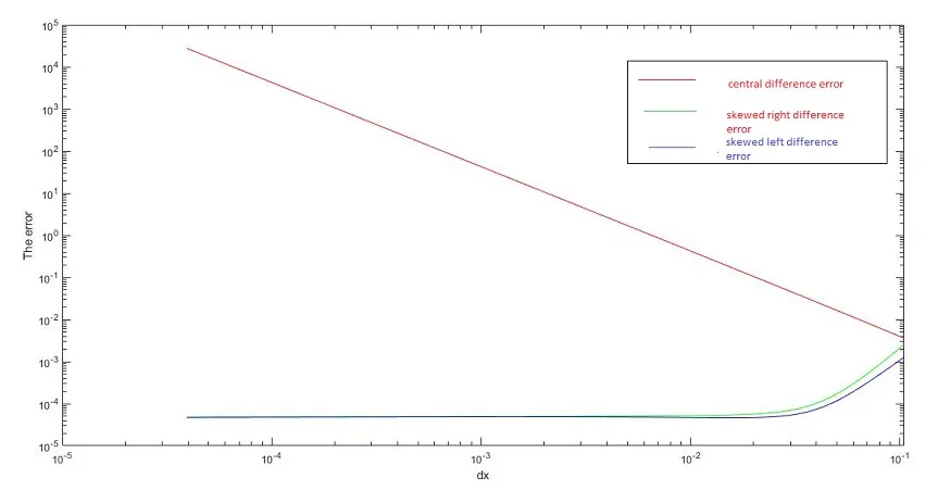
The above plot shows comparison of the fourth order approximation schemes for a range of dx. From the graph it is very clear that the highest error is observed with the central difference scheme whereas, boththe right and left skewed fourth order approximation schemes have a similar error pattern. The highest error of the central difference scheme is attributed to the fact that it uses less number of information from the points near the point under consideration. The skewed difference schemes use 'p+q' method where p(order of the derivative of the function)=2 and q(accuracy required)=4.

As the range of dx increases, the error in the central scheme starts to decrease whereas the error from the skewed schemes starts increasing.