Week 3 - Taylor table method and Matlab code

Let p=Order of the derivative

     q=Order of the error

For a central difference scheme, number of nodes required are `p+q-1`

For a skewed scheme, number of nodes required are `p+q`

• Central difference
  

The below is Taylor table for finding `4^(th)` order approximation of second order derivative using central difference method.

	`f(i)`	`(Deltax)f^1(i)`	`(Deltax)^2f^2(i)`	`(Deltax)^3f^3(i)`	`(Deltax)^4f^4(i)`	`(Deltax)^5f^5(i)`	`(Deltax)^6f^6(i)`
`af(i-2)`	a	`(-2)/(1!)a`	`(-2)^2/(2!)a`	`(-2)^3/(3!)a`	`(-2)^4/(4!)a`	`(-2)^5/(5!)a`	`(-2)^6/(6!)a`
`bf(i-1)`	b	`(-1)/(1!)b`	`(-1)^2/(2!)b`	`(-1)^3/(3!)b`	`(-1)^4/(4!)b`	`(-1)^5/(5!)b`	`(-1)^6/(6!)b`
`cf(i)`	c	0	0	0	0	0	0
`df(i+1)`	d	`(1)/(1!)d`	`(1)^2/(2!)d`	`(1)^3/(3!)d`	`(1)^4/(4!)d`	`(1)^5/(5!)d`	`(1)^6/(6!)d`
`ef(i+2)`	e	`(2)/(1!)e`	`(2)^2/(2!)e`	`(2)^3/(3!)e`	`(2)^4/(4!)e`	`(2)^5/(5!)e`	`(2)^6/(6!)e`
	0	0	1	0	0	?	?

The following are the system of equations to solve:

`[[1, 1, 1,1,1],[-2, -1,0,1,2],[2,0.5,0,0.5,2],[-8/(6),-1/6,0,1/6,8/6],[16/24,1/24,0,1/24,16/24] ]*[[a],[b],[c],[d],[e]]=[[0],[0],[1],[0],[0]]`

The following is the code to obtaion fractional values of a,b,c,d and e

clc
A=[1, 1, 1,1,1;-2, -1,0,1,2;2,1/2,0,1/2,2;-8/(6),-1/6,0,1/6,8/6;16/24,1/24,0,1/24,16/24]
B=[0;0;1;0;0]
S=rat((A^-1)*B)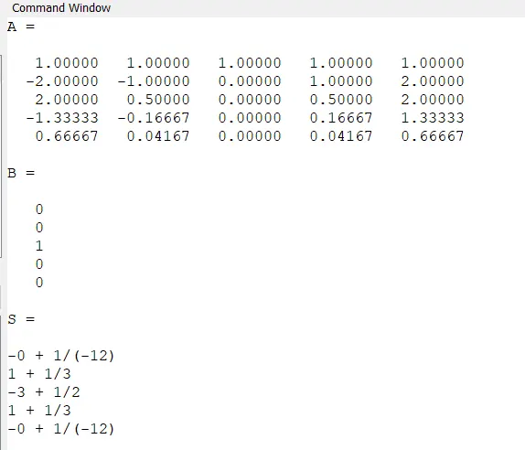

S is gives values of a,b,c,d and e. Making all the denominators of coefficients as 12 we get;

Therefore, `a=frac{-1}(12}; b=frac{16}(12} ; c=frac{-30}(12}; d=frac{16}(12}; e=frac{-1}(12}`

We can compute the coefficients of `(Deltax)^5f^5(i)` and `(Deltax)^6f^6(i)`. Since, a=e and b=d, coefficient of of `(Deltax)^5f^5(i)` is zero. 

The coefficient of `(Deltax)^6f^6(i)` is 1/90(non-zero). Hence, the order of truncation error is `(Deltax)^(6-2)=(Deltax)^(4)`

Therfore, 

`(Deltax)^2(d^2f)/(dx^2) = (-f(i-2)+16f(i-1)-30*f(i)+16f(i+1)-f(i+2))/(12) +O ((Deltax)^6)`

`(d^2f)/(dx^2) = (-f(i-2)+16f(i-1)-30f(i)+16f(i+1)-f(i+2))/(12*(Deltax)^2) +O ((Deltax)^4)`

•  Skewed right-side difference

The below is Taylor table for finding `4^(th)` order approximation of second order derivative using skewed right side scheme .

	`f(i)`	`(Deltax)f^1(i)`	`(Deltax)^2f^2(i)`	`(Deltax)^3f^3(i)`	`(Deltax)^4f^4(i)`	`(Deltax)^5f^5(i)`	`(Deltax)^6f^6(i)`
`af(i)`	a	0	0	0	0	0	0
`bf(i+1)`	b	`(1)/(1!)b`	`(1)^2/(2!)b`	`(1)^3/(3!)b`	`(1)^4/(4!)b`	`(1)^5/(5!)b`	`(1)^6/(6!)b`
`c(i+2)`	c	`(2)/(1!)c`	`(2)^2/(2!)c`	`(2)^3/(3!)c`	`(2)^4/(4!)c`	`(2)^5/(5!)c`	`(2)^6/(6!)c`
`df(i+3)`	d	`(3)/(1!)d`	`(3)^2/(2!)d`	`(3)^3/(3!)d`	`(3)^4/(4!)d`	`(3)^5/(5!)d`	`(3)^6/(6!)d`
`ef(i+4)`	e	`(4)/(1!)e`	`(4)^2/(2!)e`	`(4)^3/(3!)e`	`(4)^4/(4!)e`	`(4)^5/(5!)e`	`(4)^6/(6!)e`
`hf(i+5)`	h	`(5)/(1!)h`	`(5)^2/(2!)h`	`(5)^3/(3!)h`	`(5)^4/(4!)h`	`(5)^5/(5!)h`	`(5)^6/(6!h`
	0	0	1	0	0	0	?

The following are the system of equations to solve:

`[[1, 1, 1,1,1,1],[0,1,2,3,4,5],[0,(1)^2/2,(2)^2/2,(3)^2/2,(4)^2/2,(5)^2/2],[0,1/(3!),2^3/(3!),3^3/(3!),4^3/(3!),5^3/(3!)],[0,1^4/(4!),2^4/(4!),3^4/(4!),4^4/(4!),5^4/(4!)],[0,1^5/(5!),2^5/(5!),3^5/(5!),4^5/(5!),5^5/(5!)]]*[[a],[b],[c],[d],[e],[h]]=[[0],[0],[1],[0],[0],[0]]`

The following is the code to obtaion fractional values of a,b,c,d,e and h is as follows

clc
A=[1, 1, 1,1,1,1;0,1,2,3,4,5;0,1/2,4/2,9/2,16/2,25/2;0,1/(factorial(3)),2^3/(factorial(3)),3^3/(factorial(3)),4^3/(factorial(3)),5^3/(factorial(3));0,1^4/(factorial(4)),2^4/(factorial(4)),3^4/(factorial(4)),4^4/(factorial(4)),5^4/(factorial(4));0,1^5/(factorial(5)),2^5/(factorial(5)),3^5/(factorial(5)),4^5/(factorial(5)),5^5/(factorial(5))]
B=[0;0;1;0;0;0]
S1=((A^-1)*B)
S=rat((A^-1)*B)

The following is the screenshot of command window obtained by implementing the above code:

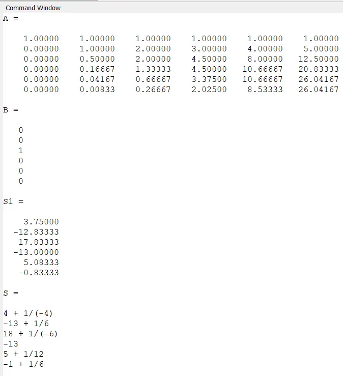
Therefore, `a=frac{45}(12}; b=frac{-154}(12} ; c=frac{214}(12}; d=frac{-156}(12}; e=frac{61}{12};e=frac{-10}{12}`

The coefficient of `(Deltax)^6f^6(i)` is non-zero. Hence, the order of truncation error is `(Deltax)^(6-2)=(Deltax)^(4)`

Therefor,

`(d^2f)/(dx^2) = (45f(i)-154f(i+1)+214f(i+2)-156f(i+3)+61f(i+4)-10f(i+5))/(12*(Deltax)^2) +O ((Deltax)^4)`

•  Skewed left-side difference

The below is Taylor table for finding `4^(th)` order approximation of second order derivative using skewed left side scheme .

	`f(i)`	`(Deltax)f^1(i)`	`(Deltax)^2f^2(i)`	`(Deltax)^3f^3(i)`	`(Deltax)^4f^4(i)`	`(Deltax)^5f^5(i)`	`(Deltax)^6f^6(i)`
`af(i)`	a	0	0	0	0	0	0
`bf(i-1)`	b	`(-1)/(1!)b`	`(-1)^2/(2!)b`	`(-1)^3/(3!)b`	`(-1)^4/(4!)b`	`(-1)^5/(5!)b`	`(-1)^6/(6!)b`
`c(i-2)`	c	`(-2)/(1!)c`	`(-2)^2/(2!)c`	`(-2)^3/(3!)c`	`(-2)^4/(4!)c`	`(-2)^5/(5!)c`	`(-2)^6/(6!)c`
`df(i-3)`	d	`(-3)/(1!)d`	`(-3)^2/(2!)d`	`(-3)^3/(3!)d`	`(-3)^4/(4!)d`	`(-3)^5/(5!)d`	`(-3)^6/(6!)d`
`ef(i-4)`	e	`(-4)/(1!)e`	`(-4)^2/(2!)e`	`(-4)^3/(3!)e`	`(-4)^4/(4!)e`	`(-4)^5/(5!)e`	`(-4)^6/(6!)e`
`hf(i-5)`	h	`(-5)/(1!)h`	`(-5)^2/(2!)h`	`(-5)^3/(3!)h`	`(-5)^4/(4!)h`	`(-5)^5/(5!)h`	`(-5)^6/(6!h`
	0	0	1	0	0	0	?

The following are the system of equations to solve:

`[[1, 1, 1,1,1,1],[0,-1,-2,-3,-4,-5],[0,(-1)^2/2,(-2)^2/2,(-3)^2/2,(-4)^2/2,(-5)^2/2],[0,(-1)^3/(3!),(-2)^3/(3!),(-3)^3/(3!),(-4)^3/(3!),(-5)^3/(3!)],[0,(-1)^4/(4!),(-2)^4/(4!),(-3)^4/(4!),(-4)^4/(4!),(-5)^4/(4!)],[0,(-1)^5/(5!),(-2)^5/(5!),(-3)^5/(5!),(-4)^5/(5!),(-5)^5/(5!)]]*[[a],[b],[c],[d],[e],[h]]=[[0],[0],[1],[0],[0],[0]]`

The following is the code to obtaion fractional values of a,b,c,d,e and h is as follows

clc
A=[1, 1, 1,1,1,1;0,-1,-2,-3,-4,-5;0,(-1)^2/2,(-2)^2/2,(-3)^2/2,(-4)^2/2,(-5)^2/2;0,(-1)^3/(factorial(3)),(-2)^3/(factorial(3)),(-3)^3/(factorial(3)),(-4)^3/(factorial(3)),(-5)^3/(factorial(3));0,(-1)^4/(factorial(4)),(-2)^4/(factorial(4)),(-3)^4/(factorial(4)),(-4)^4/(factorial(4)),(-5)^4/(factorial(4));0,(-1)^5/(factorial(5)),(-2)^5/(factorial(5)),(-3)^5/(factorial(5)),(-4)^5/(factorial(5)),(-5)^5/(factorial(5))]
B=[0;0;1;0;0;0]
S1=((A^-1)*B)
S=rat((A^-1)*B)

The following is the screenshot of command window obtained by implementing the above code:

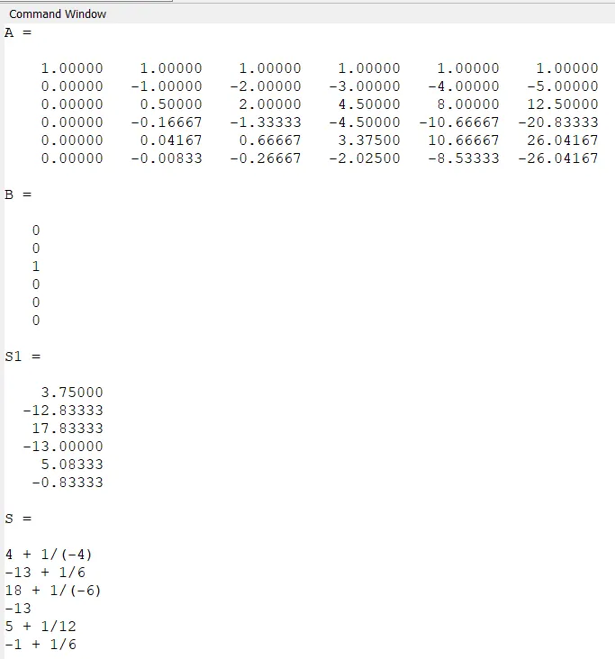
Therefore, `a=frac{45}(12}; b=frac{-154}(12} ; c=frac{214}(12}; d=frac{-156}(12}; e=frac{61}{12};e=frac{-10}{12}`

The coefficient of `(Deltax)^6f^6(i)` is non-zero. Hence, the order of truncation error is `(Deltax)^(6-2)=(Deltax)^(4)`

Therefor,

`(d^2f)/(dx^2) = (45f(i)-154f(i-1)+214f(i-2)-156f(i-3)+61f(i-4)-10f(i-5))/(12*(Deltax)^2) +O ((Deltax)^4)`

The following is the ouput of command window after running the matlab code for comparison of different scheme

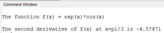
The following are the plots comparing absolute error of different schemes:

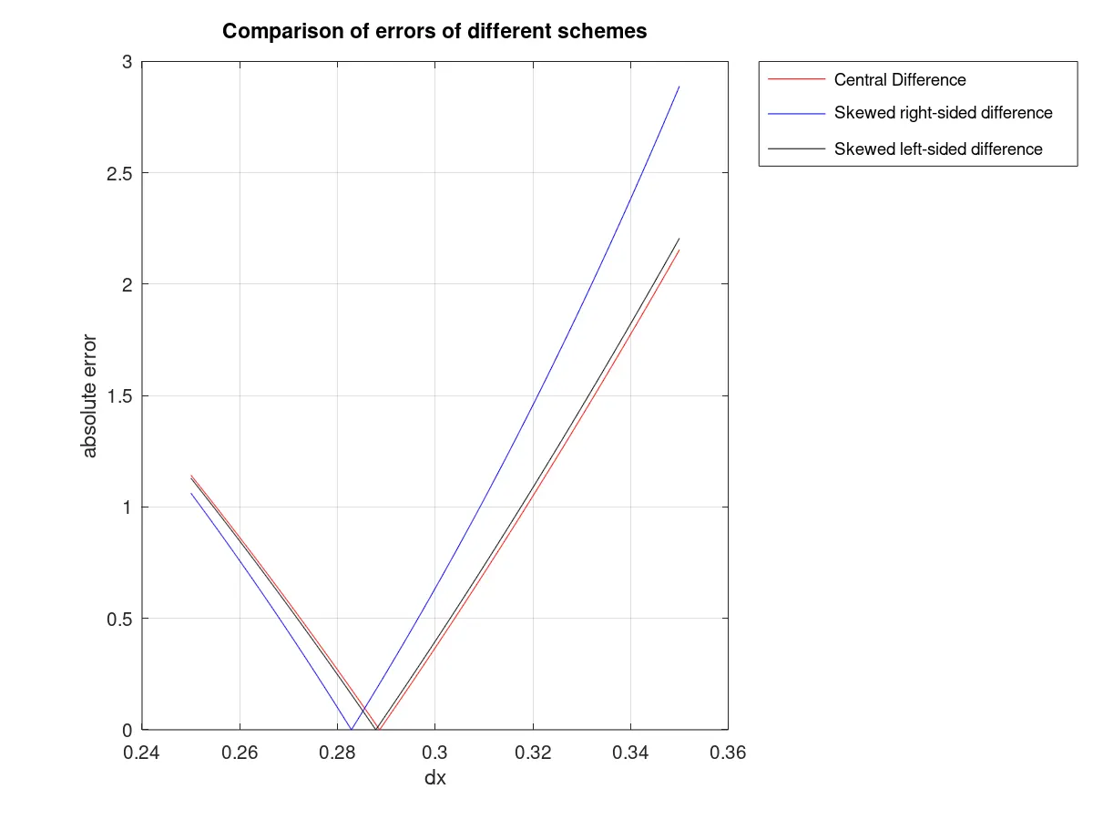
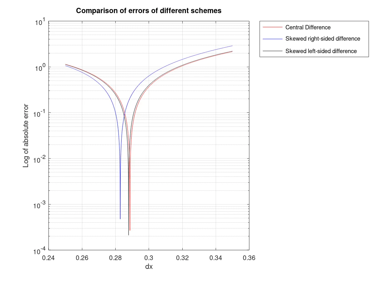
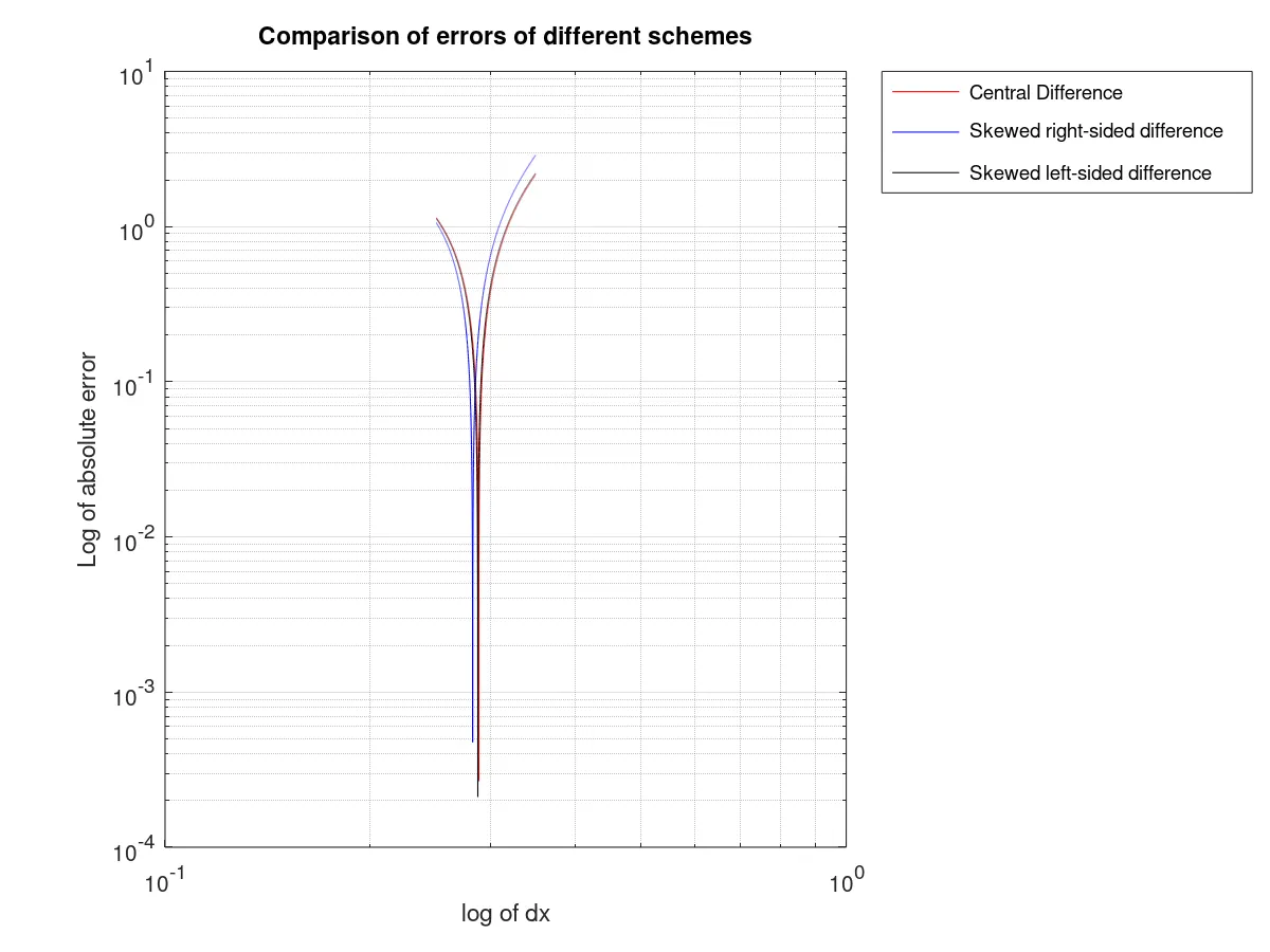
From all the above graphs, we come to know that is very limited useable range of dx to find second derivative of `e^x*cos(x)` at `x=pi/3` using the fourth order schemes.

The useable range of dx is is greater than `approx 29`. Below this value, the absolute error of   

But we cannot determine the exact range as the absolute error does not give idea of the true value at `x=pi/3`.

The relative error or relative percent error can give relative deviation of calculated value with true value.

   

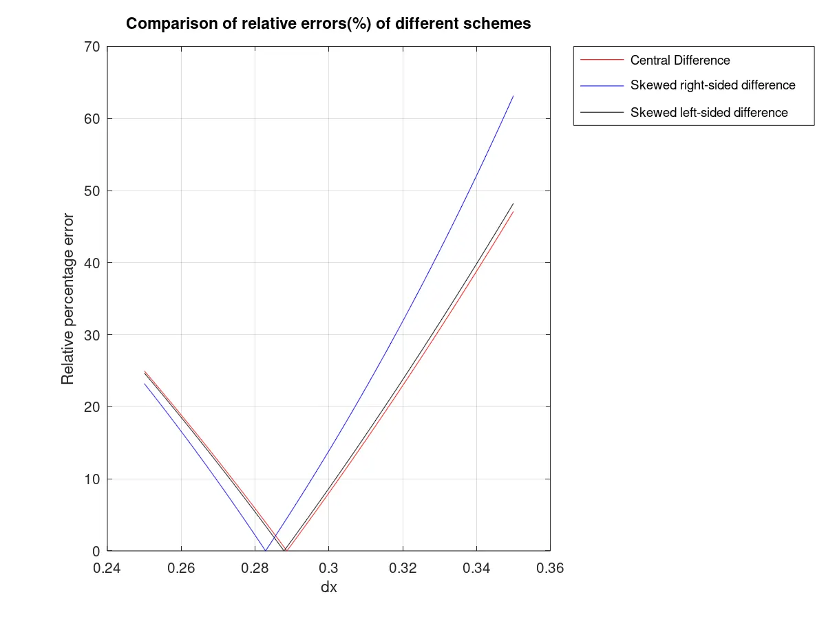
The relative percent error gives a working range based on desired accuracy of results. In any numerical calculation, the upper relative error is 30%. Relative error greater than 30% is not acceptable. 

The working range of dx is approximately from 0.29 to 0.33. In this working range, the relative error is under 30%. 

For dx>0.29, truncation error palys a dominant role.

For dx<0.29, the rounding off error plays a dominant role and hence absolute error starts increasing.

• The skewed scheme is useful to calculate value of grid points at boundary of mesh where previous or next grid points are not available. It is used to caculate value at a corner node or an edge node.
• The fourth order skewed left-side scheme is preferred over fourth order skewed right-side scheme as fourth order skewed left-side scheme is more accurate.
• The central difference scheme is preferred over a skewed scheme as takes into account the values of previous grid points as well as next grid points. The central difference scheme is more accurate than skewed scheme.   
• Order of prefererence for fourth order schemes is
  • Central difference>Skewed left-sided>Skewed right-sided

The following is the matlab code:

%Comparison of errors of central difference scheme, skewed right-sided differenece and skewed left-sided differenece
%The function f(x)=exp(x)*cos(x)
%f'(x) = exp(x)*cos(x)-exp(x)*sin(x)
%f"(x) = exp(x)*cos(x)-exp(x)*sin(x)+exp(x)*sin(x)-exp(x)*cos(x)
%Therfore, f"(x) = -2*exp(x)*sin(x)
%Find the value of x=pi/3
clc
clear all
close all
x=1;
dx=linspace(0.25,0.35,1000);
analytical_derivative = -2*exp(x)*sin(x);
e = zeros(length(dx),3);
for i=1:length(dx)
  [e(i,1) e(i,2) e(i,3)]= e2(x, dx(1,i));
end
clc
##e(i,1) = absolute error from fourth order central difference scheme
##e(i,2) = absolute error from fourth order skewed right-side difference scheme
##e(i,3) = absolute error from fourth order skewed left-side difference scheme
##Relative Percentage Error = (Absolute Error/True Value)*100
##In our case true value is analytical_derivative
rel_e = e.*(100)./(abs(analytical_derivative)); %This matrix gives the relative percentage error. 
##rel_e(i,1) = relative error(%) from fourth order central difference scheme
##rel_e(i,2) = relative error(%) from fourth order skewed right-side difference scheme
##rel_e(i,3) = relative error(%) from fourth order skewed left-side difference scheme
fprintf("\nThe function f(x) = exp(x)*cos(x)\n")
fprintf("\nThe second derivative of f(x) at x=pi/3 is %d\n",analytical_derivative) %Value of analytical derivative
figure(1)
plot(dx,e(:,1),'r',dx,e(:,2),'b',dx,e(:,3),'k')%
xlabel('dx');
ylabel('absolute error')
legend('Central Difference','Skewed right-sided difference','Skewed left-sided difference','location','northeastoutside'); 
grid on 
title('Comparison of errors of different schemes')
figure(2)
semilogy(dx,e(:,1),'r',dx,e(:,2),'b',dx,e(:,3),'k')%
xlabel('dx');
ylabel('Log of absolute error')
legend('Central Difference','Skewed right-sided difference','Skewed left-sided difference','location','northeastoutside'); 
grid on 
title('Comparison of errors of different schemes')
figure(3)
loglog(dx,e(:,1),'r',dx,e(:,2),'b',dx,e(:,3),'k')%
xlabel('log of dx');
ylabel('Log of absolute error')
legend('Central Difference','Skewed right-sided difference','Skewed left-sided difference','location','northeastoutside'); 
grid on 
title('Comparison of errors of different schemes')
figure(4)
plot(dx,rel_e(:,1),'r',dx,rel_e(:,2),'b',dx,rel_e(:,3),'k')
xlabel('dx');
ylabel('Relative percentage error')
legend('Central Difference','Skewed right-sided difference','Skewed left-sided difference','location','northeastoutside'); 
grid on 
title('Comparison of relative errors(%) of different schemes')

The following is the function'e2' used to calculate absolute error:

function [value_1 value_2 value_3] = e2 (x, dx)
  analytical_derivative = -2*exp(x)*sin(x);
  A = [exp(x-2*dx)*cos(x-2*dx) exp(x-dx)*cos(x-dx) exp(x)*cos(x) exp(x+dx)*cos(x+dx) exp(x+2*dx)*cos(x+2*dx)];
  B = [-1;16;-30;16;-1]; %Coefficients calculated fro fourth order central difference scheme
  value_1 = abs(analytical_derivative-A*B) %absolute error from fourth order central difference scheme
  C = [exp(x)*cos(x) exp(x+dx)*cos(x+dx) exp(x+2*dx)*cos(x+2*dx) exp(x+3*dx)*cos(x+3*dx) exp(x+4*dx)*cos(x+4*dx) exp(x+5*dx)*cos(x+5*dx)];
  D = [45;-154;214;-156;61;-10]; %Coefficients calculated fro fourth order skewd right-sided difference scheme
  value_2 = abs(analytical_derivative-C*D) %absolute error from fourth order skewed right-side difference scheme  
  E = [exp(x)*cos(x) exp(x-dx)*cos(x-dx) exp(x-2*dx)*cos(x-2*dx) exp(x-3*dx)*cos(x-3*dx) exp(x-4*dx)*cos(x-4*dx) exp(x-5*dx)*cos(x-5*dx)];
  F = [45;-154;214;-156;61;-10]; %Coefficients calculated fro fourth order skewd left-sided difference scheme
  value_3 = abs(analytical_derivative-E*F) %absolute error from fourth order skewed left-side difference scheme
endfunction