Week 3 - Taylor table method and Matlab code

MATLAB has been used for programming

NOTE - In this document, the forward difference scheme refers to the fourth-order skewed right side scheme and the backward difference scheme refers to the fourth-order left side scheme.

1. Derivation of the fourth-order discretization schemes for the second derivative by using the Taylor table method.

1.a. Central difference scheme

Consider that on a numerical stencil, it is of interest to calculate the second derivative of a function at node i. In order to do obtain a fourth order central difference scheme, it is necessary to consider two successive nodes on either side of the node i. Thus, the nodes, i-2, i-1, i, i+1 and i+2 are considered. The value of the independent variable at the node i is x. Let us consider the grid element size to be dx. The hypothesis equation is given as follows:

`\frac{d^2 f}{dx^2}=af_{i-2}+bf_{i-1}+cf_i+df_{i+1}+ef_{i+2}`

This can also be written as:

`\frac{d^2 f}{dx^2}=af(x-2dx)+bf(x-dx)+cf(x)+df(x+dx)+ef(x+2dx)`

The functions at nodes i-2, i-1, i+1 and i+2 are evaluated by using the Taylor series approximation. This is carried out as shown below:

`f(x-2dx)=f(x)-(2dx)f'(x)+\frac{(4dx^2)f''(x)}{2!}-\frac{(8dx^3)f'''(x)}{3!}+\frac{(16dx^4)f^{IV}(x)}{4!}-\frac{(32dx^5)f^V(x)}{5!}+\frac{(64dx^6)fVI(x)}{6!}+HOT`

The reason for choosing to expand the taylor series until the seventh term will be stated later. In a similar fashion, the taylor series expansion for the functions at i-1,i+1 and i+2 are to be written. These are further added by multiplying the coefficcients in order to obtain the hypothesis equation given earlier. This analysis can be simplified by tabulating the coefficcients in a table which is called a Taylor Table. It is done as shown below:

	f(x)	dxf'(x)	`dx^2 f''(x)`	`dx^3 f'''(x)`	`dx^4 f^(IV)(x)`	`dx^5 f^(V)(x)`	`dx^6 f^(VI)(x)`
af(x-2dx)	a	-2a	4a/2	-8a/6	16a/24	-32a/120	64a/720
bf(x-dx)	b	-b	b/2	-b/6	b/24	-b/120	b/720
cf(x)	c	0	0	0	0	0	0
df(x+dx)	d	d	d/2	d/6	d/24	d/120	d/720
ef(x+2dx)	e	2e	4e/2	8e/6	16e/24	32e/120	64e/720
Sum	0	0	1	0	0	?	?

Upon substituting for f(x-2dx), f(x-dx), f(x+dx) and f(x+2dx) in the hypothesis equation. The following is obtained:

`\frac{d^2 f}{dx^2}=(a+b+c+d+e)f(x)+(-2a-b+d+22)dxf'(x)+(2a+b/2+d/2+2e)dx^2 f''(x)+({-4a}/3-b/6+d/6+{4e}/3)dx^3 f'''(x) + _`

`({2a}/3+b/24+d/24+{2e}/3)dx^4f^{IV}(x)+({-4a}/15-b/120+d/120+{4e}/15)dx^5 f^{V}(x)+({4a}/45+b/720+d/720+{4e}/45)f^{VI}(x)`

The coefficcients of terms f(x), f'(x), f''(x), f'''(x) and `f^{IV}(x)` are equated to the corresponding numbers given in the row called sum in the taylor table. This leads to the following system of linear equations:

`a+b+c+d+e=0`

`-2a-b+d+2e=0`

`2a+b/2+d/2+2e=1`

`{-4a}/3-b/6+d/6+{4e}/3=0`

`{2a}/3+b/24+d/24+{2e}/3=0`

The system of equations can be solved using the matrix inversion method to obtain the coefficients for the hypothesis equation. The quation is converted into a simple equation in matrices as shown below:

`A X=B`

In the above equation, A is the matrix of coefficcients, X is the matrix of the coefficients of the hypothesis equation. They are defined as follows:

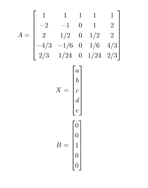
X can be obtained as follows:

`X=A^{-1}B`

The script used in Matlab to obtain the solution is as shown below:

% To calculate the coefficients for the fourth order central difference scheme by solving a system of equations obtained from the Taylor's Table %
% hypothesis function - f''(x)=af(i-2)+bf(i-1)+cf(i)+df(i+1)+ef(i+2) %
clear all
close all
clc
% Coefficient matrix %
A=[1 1 1 1 1;-2 -1 0 1 2;2 1/2 0 1/2 2;-4/3 -1/6 0 1/6 4/3;2/3 1/24 0 1/24 2/3];
B=[0;0;1;0;0];
X= inv(A)*B; % X = [a b c d e] i.e. the matrix of coefficients %
disp(X)

Logic:

The matrix of coefficients and the matrix of RHS values are defined as per the taylor table method and the inv() command is used to obtain `A^{-1)`.

The coefficients of the hypothesis equation are obtained and are as shown below.

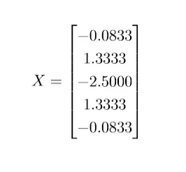
As a result of this solution, the expression preceding the term `dx^5 f^V(x)` in the Taylor approximate hypothesis equation will be zero because, `{-4a}/15-b/120+d/120+{4e}/15=0`. The resulting Taylor approximate hypothesis equation is as shown below:

`af(x-2dx)+bf(x-dx)+cf(x)+df(x+dx)+ef(x+2dx)=(2a+b/2+d/2+2e)dx^2 f''(x)+({4a}/45+b/720+d/720+{4e}/45)dx^6f^{VI}`

As we are interested in finding f''(x), the above correlation can be written as follows:

`af(x-2dx)+bf(x-dx)+cf(x)+df(x+dx)+ef(x+2dx)=(2a+b/2+d/2+2e)dx^2 f''(x)+O(dx^6)`

The term `O(dx^6)` is the truncation error term, it is not necessary to evaluate its prefactor. By dividing the above equation by dx^2 , it can be seen that the resulting correlation shows an error that is of the fourth order:

`\frac{af(x-2dx)+bf(x-dx)+cf(x)+df(x+dx)+ef(x+2dx)}{dx^2)=(2a+b/2+d/2+2e) f''(x)+O(dx^4)`

The coefficients (elements of matrix X_ are substituted in the hypothesis equation to obtain the final correlation for the fourth-order central difference scheme as shown below.

`{d^2 f}/{dx^2}=\frac{-0.0833f(x-2dx)+1.3333f(x-dx)-2.5f(x)+1.3333f(x+dx)-0.0833f(x+2dx)}{dx^2}`

1.b. Skewed Right Side Scheme (Fourth order forward difference scheme):

The skewed right side scheme is defined in a similar manner as the central difference scheme. However, five nodes ahead of the node of interest are chosen in order to evaluate the second derivative. Following is the hypothesis equation for the skewed right side scheme:

`\frac{d^2 f}{dx^2}=af_{i}+bf_{i+1}+cf_{i+2}+df_{i+3}+ef_{i+4}+gf_{i+5}`

Which can also be written as:

`\frac{d^2 f}{dx^2}=af(x)+bf(x+dx)+cf(x+2dx)+df(x+3dx)+ef(x+4dx)+gf(x+5dx)`

The Taylor Table for the above hypothesis equation is as follows:

	f(x)	dx f'(x)	`dx^2 f''(x)`	`dx^3 f'''(x)`	`dx^4 f^{IV}(x)`	`dx^5 f^V(x)`	`dx^6 f^{VI}(x)`
f(i)	a	0	0	0	0	0	0
f(i+1)	b	b	b/2	b/6	b/24	b/120	b/720
f(i+2)	c	2c	4c/2	8c/6	16c/24	32c/120	64c/720
f(i+3)	d	3d	9d/2	27d/6	81d/24	243d/120	729c/720
f(i+4)	e	4e	16e/2	64e/6	256e/24	1024e/120	4096e/720
f(i+5)	g	5g	25g/2	125g/6	625g/24	3125g/120	15625e/720
	0	0	1	0	0	0	?

The following simultaneous equations have to be solved in order to obtain the coefficients for the hypothesis equation.

`a+b+c+d+e+g=0`

`b+2c+3d+4e+5g=0`

`b/2+2c+9d/2+8e+25g/2=1`

`b/6+{8c}/6+{9d}/2+{32e}/3+{125g}/6=0`

`b/24+{2c}/3+{27d}/8+{32e}/3+{625g}/24=0`

`b/120+{4c}/15+{81d}/40+{128e}/15+{625g}/24=0`

The system of equations can be solved using the matrix inversion method to obtain the coefficients for the hypothesis equation. The equation is converted into a simple equation in matrices as shown below:

`A X=B`

In the above equation, A is the matrix of coefficients, X is the matrix of the coefficients of the hypothesis equation. They are defined as follows:

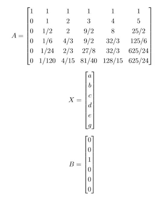
X can be obtained as follows:

`X=A^{-1}B`

The script used in Matlab to obtain the solution is as shown below:

% To calculate the coefficients for the fourth order forward difference skewed scheme by solving a system of equations obtained from the Taylor's Table %
clear all
close all
clc
% Coefficient matrix %
A=[1 1 1 1 1 1; 0 1 2 3 4 5; 0 1/2 2 9/2 8 25/2; 0 1/6 4/3 9/2 32/3 125/6; 0 1/24 2/3 27/8 32/3 625/24; 0 1/120 4/15 81/40 128/15 625/24];
B=[0;0;1;0;0;0];
X= inv(A)*B; % X = [a b c d e g] i.e. the matrix of coefficients %
disp(X)

The coefficients of the hypothesis equation are obtained and are as shown below.

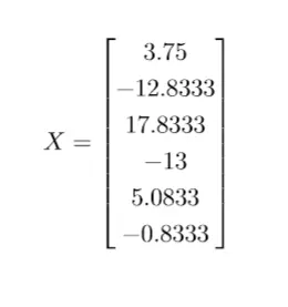
The resulting Taylor approximate hypothesis equation is as shown below:

`af(x)+bf(x+dx)+cf(x+2dx)+df(x+3dx)+ef(x+4dx)+gf(x+5dx)=(b/2+2c+{9d}/2+8e+{25g}/2)dx^2 f''(x)+O(dx^6)`

This is because the prefactors of the terms involving f'(x), f'''(x),`f^{IV}(x)`and `f^V(x)`are zero and the prefactor for the term `dx^2 f''(x)`is unity. Dividing the above expression by dx^2 on either side, we get the hypothetical equation for the second derivative and is of the fourth order.

`\frac{af(x)+bf(x+dx)+cf(x+2dx)+df(x+3dx)+ef(x+4dx)+gf(x+5dx)}{dx^2}= f''(x)+O(dx^4)`

By substituting the coefficients (elements of X) in the above correlation, we will get the numerical approximate of the second derivative by the skewed right sided difference.

`\frac{d^2 f}{dx^2}=\frac{3.75f(x)-12.8333f(x+dx)+17.8333f(x+2dx)-13f(x+3dx)+5.0833f(x+4dx)-0.8333f(x+5dx)}{dx^2}= f''(x)+O(dx^4)`

1.c. Skewed Left Side Scheme (Fourth order backward difference scheme):

The skewed left side scheme is defined in a similar manner as the central difference scheme. However, five nodes behind the node of interest are chosen in order to evaluate the second derivative. Following is the hypothesis equation for the skewed right side scheme:

`\frac{d^2 f}{dx^2}=af_{i-5}+bf_{i-4}+cf_{i-3}+df_{i-2}+ef_{i-1}+gf_{i}`

Which can also be written as:

`\frac{d^2 f}{dx^2}=af(x-5dx)+bf(x-4dx)+cf(x-3dx)+df(x-2dx)+ef(x-dx)+gf(x)`

The Taylor Table for the above hypothesis equation is as follows:

	f(x)	dx f'(x)	`dx^2 f''(x)`	`dx^3 f'''(x)`	`dx^4 f^{IV}(x)`	`dx^5 f^{V}(x)`	`dx^6 f^{VI}(x)`
f(i-5)	a	-5a	25a/2	-125a/6	625a/24	-3125a/120	15625a/720
f(i-4)	b	-4b	16b/2	-64b/6	256b/24	-1024b/120	4096b/720
f(i-3)	c	-3c	9c/2	-27c/6	81c/24	-234c/120	729c/720
f(i-2)	d	-2d	4d/2	-8d/6	16d/24	-32d/120	64d/720
f(i-1)	e	-e	e/2	-e/6	e/24	-e/120	e/720
f(i)	g	0	0	0	0	0	0
	0	0	1	0	0	0	?

The following simultaneous equations have to be solved in order to obtain the coefficients for the hypothesis equation.

`a+b+c+d+e+g=0`

`-5a-4b-3c-2d-e=0`

`{25a}/2+{8b}/2+{9c}/2+2d+e/2=0`

`-{125a}/6-{32b}/3-{9c}/2-{4e}/3-e/6=0`

`{625a}/24+{32b}/3+{27c}/8+{2d}/3+e/24=0`

`-{625a}/24-{128b}/15-{81c}/40-{4d}/15-e/120=0`

The system of equations can be solved using the matrix inversion method to obtain the coefficients for the hypothesis equation. The equation is converted into a simple equation in matrices as shown below:

`A X=B`

In the above equation, A is the matrix of coefficients, X is the matrix of the coefficients of the hypothesis equation. They are defined as follows:

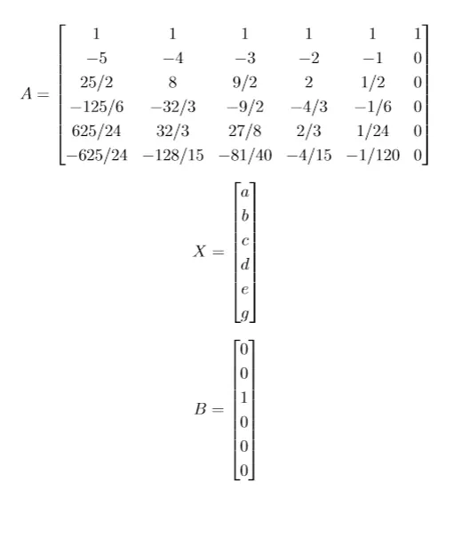
can be obtained as follows:

`X=A^{-1}B`

The script used in Matlab to obtain the solution is as shown below:

% To calculate the coefficients for the fourth order backward difference skewed scheme by solving a system of equations obtained from the Taylor's Table %
% hypothesis function -  %
clear all
close all
clc
% Coefficient matrix %
A=[1 1 1 1 1 1; -5 -4 -3 -2 -1 0; 25/2 8 9/2 2 1/2 0; -125/6 -32/3 -9/2 -4/3 -1/6 0; 625/24 32/3 27/8 2/3 1/24 0; -625/24 -128/15 -81/40 -4/15 -1/120 0];
B=[0;0;1;0;0;0];
X= inv(A)*B; % X = [a b c d e g] i.e. the matrix of coefficients %
disp(X)

The coefficients of the hypothesis equation are obtained and are as shown below.

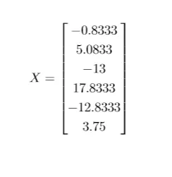
The resulting Taylor approximate hypothesis equation is as shown below:

`af(x-5dx)+bf(x-4dx)+cf(x-3dx)+df(x-2dx)+ef(x-dx)+gf(x)=({25a}/2+8b+{9c}/2+2d+e/2)dx^2 f''(x)+O(dx^6)`

This is because the prefactors of the terms involving f'(x), f'''(x),`f^{IV}(x)`and `f^V(x)`are zero and the prefactor for the term `dx^2 f''(x)`is unity. Dividing the above expression by dx^2 on either side, we get the hypothetical equation for the second derivative and is of the fourth order.

`\frac{af(x-5dx)+bf(x-4dx)+cf(x-3dx)+df(x-2dx)+ef(x-dx)+gf(x)}{dx^2}=f''(x)+O(dx^4)`

By substituting the coefficients (elements of X) in the above correlation, we will get the numerical approximate of the second derivative by the skewed right sided difference.

`{d^2 f}/{dx^2}=\frac{-0.8333f(x-5dx)+5.0833f(x-4dx)-13f(x-3dx)+17.8333f(x-2dx)-12.8333f(x-dx)+3.75f(x)}{dx^2}=f''(x)+O(dx^4)`

Let us compare the three different numerical second derivatives with the analytical second derivative of the function exp(x)*cos(x). The analytical second derivative is as follows:

`\frac{d^2f}{df^2}=-2e^x sinx`

Following is a program to visualize the function curve of the analytical and the numerically approximate second derivatives:

% Comparison of the analytical derivative with the numerically approximated second derivative %
clear all
close all
clc
syms x
dx=pi/5;
% function : f(x) = exp(x)*cos(x) %
% analytical second derivative: f"(x)=-2*exp(x)*sin(x) %
analytical= -2*exp(x)*sin(x);
% Coefficients of the hypothesis equation for the fourth order backward difference skewed scheme %
z(:,1)=[-0.8333;5.0833;-13;17.8333;-12.8333;3.7500];
% Coefficients of the hypothesis equation for the fourth order forward difference skewed scheme %
z(:,2)=[3.75;-12.8333;17.8333;-13;5.0833;-0.8333];
% Coefficients of the hypothesis equation for the fourth order central difference scheme %
z(:,3)=[-0.0833;1.3333;-2.5;1.3333;-0.0833;0];
% z is a matrix of the coefficcients of the hypothesis equation for the different discretization schemes %
% second derivative based on fourth order central difference scheme %
central=((z(1,3)*exp(x-2*dx)*cos(x-2*dx))+(z(2,3)*exp(x-dx)*cos(x-dx))+(z(3,3)*exp(x)*cos(x))+(z(4,3)*exp(x+dx)*cos(x+dx))+(z(5,3)*exp(x+2*dx)*cos(x+2*dx)))/(dx^2);
% second derivative based on fourth order forward difference scheme %
forward=((z(1,2)*exp(x)*cos(x))+(z(2,2)*exp(x+dx)*cos(x+dx))+(z(3,2)*exp(x+2*dx)*cos(x+2*dx))+(z(4,2)*exp(x+3*dx)*cos(x+3*dx))+(z(5,2)*exp(x+4*dx)*cos(x+4*dx))+(z(6,2)*exp(x+5*dx)*cos(x+5*dx)))/(dx^2);
% second derivative based on fourth order backward difference scheme %
backward=((z(1,1)*exp(x-5*dx)*cos(x-5*dx))+(z(2,1)*exp(x-4*dx)*cos(x-4*dx))+(z(3,1)*exp(x-3*dx)*cos(x-3*dx))+(z(4,1)*exp(x-2*dx)*cos(x-2*dx))+(z(5,1)*exp(x-dx)*cos(x-dx))+(z(6,1)*exp(x)*cos(x)))/(dx^2);
% plotting the figure comparing the analytical and numerical approximate second derivatives with a mesh size of pi/50 %
fplot(analytical,'-*')
hold on
fplot(central,'-o')
hold on
fplot(forward)
hold on
fplot(backward,'-^')
hold on
ylabel('f"(x)')
xlabel('x')
legend('Analytical Derivative','Fourth Order Central Difference','Fourth Order Forward Difference','Fourth Order Backward Difference','Location','southwest')
xlim([-10 15])
ylim([-300 300])
hold off

Logic:

Initially, x is defined as an independent variable. The second derivative is evaluated for a case on a numerical stencil with the element size (dx) of pi/5. The coefficients of the hypothesis equations for all the three schemes are deefined in the array z. The hypothetical equations are defined for all the three schemes. Finally, the analytical and the numerically approximate derivatives are plotted by using the appropriate plotting commands.

Output:

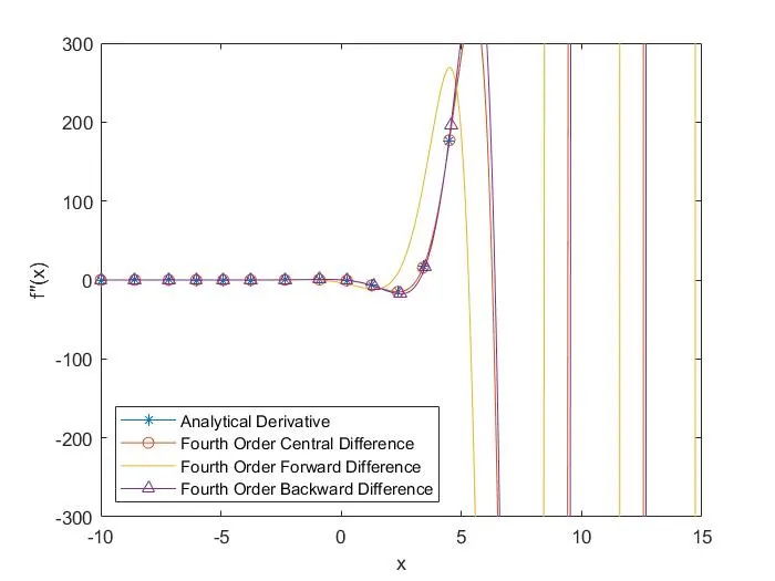
It can be seen in the above figure that for a range of x, all the three numerically approximate derivatives are reasonably accurate. However, after a certain point after x=0, the numerically approximate derivatives deviate from the analytical derivative with the fourth-order central difference scheme the most offset from the analytical derivative. Whereas the curve for the forward (or skewed right side) difference and the backward (or skewed left side) difference still matches the analytical derivative albeit with some amount of error. This error can, however, be reduced by decreasing the mesh/grid size. This is shown in the next section.

2. Comparing the Truncation Error between the three schemes:

The truncation error is the absolute value of the difference between the analytical derivative and the numerical approximations. The truncation error for all the three schemes is defined in function files as shown below.

Function file for the truncation error of the fourth-order central difference scheme:

function truncation_error=fourth_order_central_difference(x,dx,z)
% function : f(x)=exp(x)*cos(x) %
% analytical second derivative : f"(x) = -2*exp(x)*sin(x) %
analytical = -2*exp(x)*sin(x);
% fourth order central difference scheme : f"(x) = (a(3)*f(i-2)+b(3)*f(i-1)+c(3)*f(i)+d(3)*f(i)+e(3)*f(i+1)+g(3)*f(i+2))/(dx^2) %
central_difference=((z(1,3)*exp(x)*cos(x))+(z(2,3)*exp(x+dx)*cos(x+dx))+(z(3,3)*exp(x+2*dx)*cos(x+2*dx))+(z(4,3)*exp(x+3*dx)*cos(x+3*dx))+(z(5,3)*exp(x+4*dx)*cos(x+4*dx))+(z(6,3)*exp(x+5*dx)*cos(x+5*dx)))/(dx^2);
%truncation error is the absolute value of the difference between the analytical derivative and the approximation %
truncation_error = abs(central_difference - analytical);

Function file for the truncation error of the fourth-order forward (right side skewed) difference scheme:

function truncation_error=fourth_order_forward(x,dx,z)
% function : f(x)=exp(x)*cos(x) %
% analytical second derivative : f"(x) = -2*exp(x)*sin(x) %
analytical = -2*exp(x)*sin(x);
% fourth order forward difference scheme : f"(x) = (a(1)*f(i)+b(1)*f(i+1)+c(1)*f(i+2)+d(1)*f(i+3)+e(1)*f(i+4)+g(1)*f(i+5))/(dx^2) %
forward_difference=((z(1,2)*exp(x)*cos(x))+(z(2,2)*exp(x+dx)*cos(x+dx))+(z(3,2)*exp(x+2*dx)*cos(x+2*dx))+(z(4,2)*exp(x+3*dx)*cos(x+3*dx))+(z(5,2)*exp(x+4*dx)*cos(x+4*dx))+(z(6,2)*exp(x+5*dx)*cos(x+5*dx)))/(dx^2);
%truncation error is the absolute value of the difference between the analytical derivative and the approximation %
truncation_error = abs(forward_difference - analytical);

Function file for the truncation error of the fourth-order backward (left side skewed) difference scheme:

function truncation_error=fourth_order_backward(x,dx,z)
% function : f(x)=exp(x)*cos(x) %
% analytical second derivative : f"(x) = -2*exp(x)*sin(x) %
analytical = -2*exp(x)*sin(x);
% fourth order backward difference scheme : f"(x) = (a(1)*f(i-5)+b(1)*f(i-4)+c(1)*f(i-3)+d(1)*f(i-2)+e(1)*f(i-1)+g(1)*f(i))/(dx^2) %
backward_difference=((z(1,1)*exp(x-5*dx)*cos(x-5*dx))+(z(2,1)*exp(x-4*dx)*cos(x-4*dx))+(z(3,1)*exp(x-3*dx)*cos(x-3*dx))+(z(4,1)*exp(x-2*dx)*cos(x-2*dx))+(z(5,1)*exp(x-dx)*cos(x-dx))+(z(6,1)*exp(x)*cos(x)))/(dx^2);
%truncation error is the absolute value of the difference between the analytical derivative and the approximation %
truncation_error = abs(backward_difference - analytical);

Logic of the function files:

The function is defined to expect inputs of x, mesh size dx and the coefficients of the hypothesis equation (z, which is defined in the main script) for the numerically approximate second derivative. The analytical and numerical second-order derivatives are defined and this is followed by the definition of the truncation error. These functions are then called in the main script which compares the truncation errors of all the three schemes.

Main Script to compare the truncation error of the discretization schemes:

% Comparing the truncation error of the different schemes  %
clear all
close all
clc
% Linear range of mesh sizes is given by array dx%
dx=linspace(pi/3,pi/5000,80);
x=pi/4; % second derivative is calculated at point pi/6 %
% Coefficients of the hypothesis equation for the fourth order backward difference skewed scheme %
z(:,1)=[-0.8333;5.0833;-13;17.8333;-12.8333;3.7500];
% Coefficients of the hypothesis equation for the fourth order forward difference skewed scheme %
z(:,2)=[3.75;-12.8333;17.8333;-13;5.0833;-0.8333];
% Coefficients of the hypothesis equation for the fourth order central difference scheme %
z(:,3)=[-0.0833;1.3333;-2.5;1.3333;-0.0833;0];
% z is a matrix of the coefficcients of the hypothesis equation for the different discretization schemes %
for i=1:length(dx) % used in order to calculate the truncation error for all the different grid sizes %
    fourth_order_central_error(i)=fourth_order_central_difference(x,dx(i),z); % truncation error for the fourth order central difference scheme %
    fourth_order_forward_error(i)=fourth_order_forward(x,dx(i),z); % truncation error for the fourth order forward difference scheme %
    fourth_order_backward_error(i)=fourth_order_backward(x,dx(i),z); % truncation error for the fourth order backward difference scheme %
end
loglog(dx,fourth_order_central_error,'displayname','fourth order central','linewidth',1)
hold on
loglog(dx,fourth_order_forward_error,'displayname','fourth order forward','linewidth',1)
hold on
loglog(dx,fourth_order_backward_error,'displayname','fourth order backward','linewidth',1)
grid on
xlabel('Element size, dx')
ylabel('Truncation Error')
legend('Location','northwest')
hold off

Logic:

The different mesh sizes are allocated to the array dx. The mesh sizes are in the range of pi/3 to pi/5000. About 80 different sizes are chosen in this interval. The truncation error is calculated for the case where x=pi/4. The coefficients of the hypothesis equation for all the three numerically approximate derivatives are defined in the matrix z. A for loop with a counter which runs over the length of the array of mesh sizes is used to compute the three truncation errors for each mesh size. The function files of all the three discretization schemes are called and the truncation errors are evaluated at different mesh sizes. As the magnitude of errors varies significantly from coarse to fine grids. With the appropriate commands, a log-log plot is used to compare the variation of the truncation errors with the mesh size.

Output:

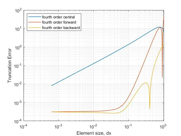
In the above figure, it can be observed that initially for a very coarse mesh, the forward difference (skewed right side scheme) scheme shows the highest truncation error which was shown in the previous image which compared the second derivatives. The backward difference (skewed right side) scheme, on the other hand, offers the least truncation error over the chosen range of mesh sizes.

In a moderately refined mesh, however, the truncation error caused by the forward scheme drops and rises rapidly over a small range of mesh sizes. In this range of mesh sizes, both the forward and the central difference scheme show comparable values of truncation errors. The error due to the forward scheme again drops considerably with the decrease in the size of the grid elements. With further refinement of the grid, the truncation error due to forward scheme gradually drops and becomes comparable to the magnitude of error due to the backward difference scheme.

The behaviour of the backward difference scheme, but the decrease in the magnitude of the truncation error is much more gradual in this case. And for very fine meshes, it can be predicted by extrapolation that all the three schemes offer comparable truncation errors.

Applicability of the different schemes:

As the central difference scheme uses information from nodes located on either side of the point of interest, it is recommended to be used in the interior parts of the domain. And as the skewed schemes require information from only one side of the node, it is recommended to use the appropriate skewed schemes based on the boundaries.

NOTE - In this document, the forward difference scheme refers to the fourth-order skewed right side scheme and the backward difference scheme refers to the fourth-order left side scheme.