Week 3 - Taylor table method and Matlab code

Taylor Tables

These schemes are derived using the taylor series expansions of a function.

`f(x+a)=(overset(infty) underset(i=0) Sigma f^i(a)*(Deltax)^i)/(a!)`

As per the given rule of including p+q number of terms in the approximation in case of a skewed scheme and p+q-1 in case of a central difference scheme.... 6 terms are included for the skewed cases and 5 terms are included for the central difference case.

p-order of derivative , q- order of approximation.

The terms included along with their expansions are given in the taylor tables.

The number of terms are 6 and 5 , therfore an equivelant number of equations are needed for solving for the coeffients . As a consequence all terms consisting of lower powers of `(Deltax)^4` are included in the taylor tables . Therefore the approximation is fourth-order accurate.

Skewed Right-sided difference

`ddotf=[ a*f(i) + b*f(i+1) + c*f(i+2) + d*f(i+3) + e*f(i+4) + g*f(i+5)]/((Deltax^2))`

	`f(i)`	`Deltax*f'(x)`	`Deltax^2*f''(x)`	`Deltax^3*f'''(i)`	`Deltax^4*f''''(i)`	`Deltax^5*f'''''(i)`
a.f(i)	a	0	0	0	0	0
b.f(i+1)	b	b	b/2	b/6	b/24	b/120
c.f(i+2)	c	2c	4c/2	8c/6	16c/24	32c/120
d.f(i+3)	d	3d	9d/2	27d/6	81d/24	243d/120
e.f(i+4)	e	4e	16e/2	64e/6	256e/24	1024e/120
g.f(i+5)	g	5g	25g/2	125g/6	625g/24	3125g/120
SUM-	0	0	1	0	0	0

Skewed Left-sided difference

`ddotf=[ a*f(i) + b*f(i-1) + c*f(i-2) + d*f(i-3) + e*f(i-4) + g*f(i-5)]/((Deltax^2))`

	`f(i)`	`Deltax*f'(x)`	`Deltax^2*f''(x)`	`Deltax^3*f'''(i)`	`Deltax^4*f''''(i)`	`Deltax^5*f'''''(i)`
a.f(i)	a	0	0	0	0	0
b.f(i+1)	b	-b	b/2	-b/6	b/24	-b/120
c.f(i+2)	c	-2c	4c/2	-8c/6	16c/24	-32c/120
d.f(i+3)	d	-3d	9d/2	-27d/6	81d/24	-243d/120
e.f(i+4)	e	-4e	16e/2	-64e/6	256e/24	-1024e/120
g.f(i+5)	g	-5g	25g/2	-125g/6	625g/24	-3125g/120
SUM-	0	0	1	0	0	0

Central Difference

`ddotf=(a.f(i-2) + b.f(i-1) + c.f(i) + d.f(i+1) + e.f(i+2))/(Deltax^2)`

	`f(i)`	`Deltax*f'(i)`	`Deltax^2*f''(i)`	`Deltax^3.f'''(i)`	`Deltax^4.f''''(i)`
a.f(i-2)	a	-2a	4a	-8a/6	16a/24
b.f(i-1)	b	-b	b/2	-b/6	b/24
c.f(i)	c	0	0	0	0
d.f(i+1)	d	d	d/2	d/6	d/24
e.f(i+2)	e	2e	4e/2	8e/6	16e/24
SUM-	0	0	1	0	0

These values are entered as matrices into MATLAB in order to solve for the coefficients. A series of values of x are taken using the 'linspace command' in order to obtain multiple values of dx=x(2)-x(1).

MAIN PROGRAM-
for i=15:1000
    x=linspace(0,10,2*i);
    dx=x(2)-x(1);
    delta_x(i-14)=dx;
    A_RS=[1 1 1 1 1 1;0 1 2 3 4 5;0 1/2 4/2 9/2 16/2 25/2; 0 1/6 8/6 27/6 64/6 125/6;0 1/24 16/24 81/24 256/24 625/24;0 1/120 32/120 243/120 1024/120 3125/120];
    A_LS=[1 1 1 1 1 1;0 -1 -2 -3 -4 -5;0 1/2 4/2 9/2 16/2 25/2; 0 -1/6 -8/6 -27/6 -64/6 -125/6;0 1/24 16/24 81/24 256/24 625/24;0 -1/120 -32/120 -243/120 -1024/120 -3125/120];
    A_CD=[1 1 1 1 1; -2 -1 0 1 2 ; 4/2 1/2 0 1/2 4/2; -8/6 -1/6 0 1/6 8/6; 16/24 1/24 0 1/24 16/24];
    B_RS=[0 ;0; 1; 0; 0; 0];
    B_LS=[0; 0; 1; 0; 0; 0];
    B_CD=[0;0;1;0;0];
    C_RS=inv(A_RS)*B_RS;
    C_LS=inv(A_LS)*B_LS;
    C_CD=inv(A_CD)*B_CD;
    K1_RS=fun(x(i));
    K2_RS=fun(x(i+1));
    K3_RS=fun(x(i+2));
    K4_RS=fun(x(i+3));
    K5_RS=fun(x(i+4));
    K6_RS=fun(x(i+5));
    K1_LS=fun(x(i));
    K2_LS=fun(x(i-1));
    K3_LS=fun(x(i-2));
    K4_LS=fun(x(i-3));
    K5_LS=fun(x(i-4));
    K6_LS=fun(x(i-5));

    ana_der= fun_der(x(i));
    num_der_RS=(K1_RS*C_RS(1) + K2_RS*C_RS(2) + K3_RS*C_RS(3) + K4_RS*C_RS(4) + K5_RS*C_RS(5) + K6_RS*C_RS(6))/(dx^2);
    num_der_LS=(K1_LS*C_LS(1) + K2_LS*C_LS(2) + K3_LS*C_LS(3) + K4_LS*C_LS(4) + K5_LS*C_LS(5) + K6_LS*C_LS(6))/(dx^2);
    num_der_CD=(K3_LS*C_CD(1) + K2_LS*C_CD(2) + K1_LS*C_CD(3) + K2_RS*C_CD(4) + K3_RS*C_CD(5))/(dx^2);
    error_RS(i-14)=abs(ana_der-num_der_RS);
    error_LS(i-14)=abs(ana_der-num_der_LS);
    error_CD(i-14)=abs(ana_der-num_der_CD);

end
figure(1)
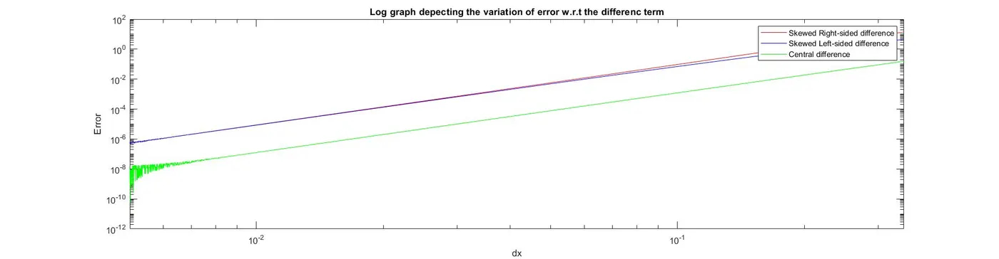
loglog(delta_x,error_RS,'r');
hold on
loglog(delta_x,error_LS,'b');
hold on
loglog(delta_x,error_CD,'g');
legend('Skewed Right-sided difference','Skewed Left-sided difference','Central difference');
title('Log graph depecting the variation of error w.r.t the differenc term');
xlabel('dx');
ylabel('Error');
set(gcf,'position',[10,10,2000,400]);
figure(2)
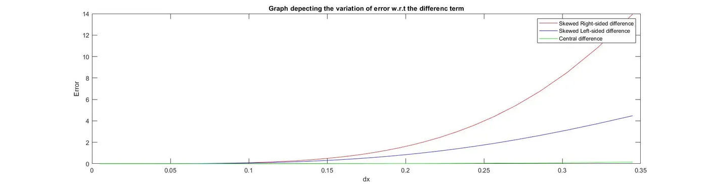
plot(delta_x,error_RS,'r');
hold on
plot(delta_x,error_LS,'b');
hold on
plot(delta_x,error_CD,'g');
legend('Skewed Right-sided difference','Skewed Left-sided difference','Central difference');
title('Graph depecting the variation of error w.r.t the differenc term');
xlabel('dx');
ylabel('Error');
set(gcf,'position',[10,10,2000,400]);

fun.m
function out = fun(x)
out =exp(x)*cos(x);
end

fun_der.m
function out =fun_der(x)
out =(-2)*(exp(x)*sin(x));
end

Graphs

Conclusion-

1.The errors in the central difference scheme are much lower than the skewed cases their rate of climb is also lower.

2.Although the central difference scheme gives a more accurate approximation it would not work for boundry cases , in which there are no nodes available on one side , since central differencing requires information from both sides , the simulation would fail in this case .

3.The skewed case an operate in a boundry condtion (right of left skewed depends on direction of flow of information) whereas a central difference cannot.