Week 3 - Taylor table method and Matlab code

Introduction:

Numerical solutioncan only give ansswers at discrete points in the domain which are called as grid points.The finite difference methods is for replacing the partial derivates appearing in governing eqaution of fluid dynamics,with algebraic difference qouitents yeilding a system of governing equations which can be solved for the flow field variables at the specific discrete grid points in the flow.

Schemes for fourth order approximations for second order derivatives:

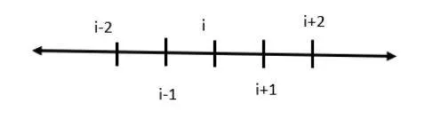
We have a set of grid points in our numerical stencil along the x-plane.Each grid point has its own taylor series functions.We first create a taylor table from these set of grid points as shown below.

1.Central difference scheme:

central differencing with fourth order approximation:

`(del^2f)/(delx^2)`=`(af(i-2)+bf(i-1)+cf(i)+df(i+1)+ef(i+2))/(Deltax^2)`

	f(i)	f'(i)*`Delta`(x)	f''(i)*`Delta`(x)^2	f'''(i)*`Delta`(x)^3	f''''(i)*`Delta`(x)^4
f(i-2)	a	-2a	4a/2	-8a/6	16a/24
f(i-1)	b	-b	b/2	-b/6	b/24
f(i)	c	0	0	0	0
f(i+1)	d	d	d/2	d/6	d/24
f(i+2)	e	2e	4e/2	8e/6	16e/24
	0	0	1	0	0

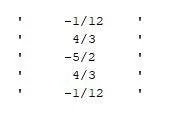
For central difference scheme all the co-efficients can be find out by using below matlab code:

E=[1 1 1 1 1;
    -2 -1 0 1 2;
    4/2 1/2 0 1/2 4/2;
    -8/6 -1/6 0 1/6 8/6;
    16/24 1/24 0 1/24 16/24];

F=[0;0;1;0;0];

Z=rats(linsolve(E,F))

Outputs:

2. Skewed right-sided difference scheme:

skewed right sided with fourth order approximation:

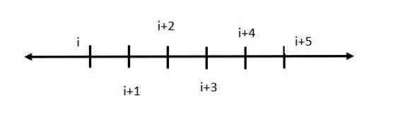
`(del^2f)/(delx^2)=(af(i)+bf(i+1)+cf(i+2)+df(i+3)+ef(i+4)+gf(i+5))/(Deltax^2)`

	f(i)	f'(i)*`Delta`(x)	f''(i)*`Delta`(x)^2	f'''(i)*`Delta`(x)^3	f''''(i)*`Delta`(x)^4	f'''''(i)*`Delta`(x)^5
f(i)	a	0	0	0	0	0
f(i+1)	b	b	b/2	b/6	b/24	b/120
f(i+2)	c	2c	4c/2	8c/6	16c/24	32c/120
f(i+3)	d	3d	9d/2	27d/6	81d/24	243d/120
f(i+4)	e	4e	16e/2	64e/6	256e/24	1024e/120
f(i+5)	g	5g	25g/2	125g/6	625g/24	3125g/120
	0	0	1	0	0	0

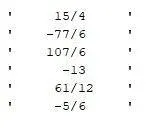
For skewed rightside difference scheme all the co-efficients can be find out by using below matlab code:

E=[1 1 1 1 1 1;
    0 1 2 3 4 5 ;
    0 1/2 4/2 9/2 16/2 25/2;
    0 1/6 8/6 27/6 64/6 125/6;
    0 1/24 16/24 81/24 256/24 625/24;
    0 1/120 32/120 243/120 1024/120 3125/120];

F=[0;0;1;0;0;0];
Z=rats(linsolve(E,F))

Outputs:

3.Skewed left-sided difference scheme:

skewed leftside difference with foruth order approximation:

`(del^2f)/(delx^2)=(af(i)+bf(i-1)+cf(i-2)+df(i-3)+ef(i-4)+gf(i-5))/(Deltax^2)`

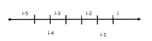
	f(i)	f'(i)*`Delta`(x)	f''(i)*`Delta`(x)^2	f'''(i)*`Delta`(x)^3	f''''(i)*`Delta`(x)^4	f'''''(i)*`Delta`(x)^5
f(i)	a	0	0	-0	0	-0
f(i-1)	b	-b	b/2	-b/6	b/24	-b/120
f(i-2)	c	-2c	4c/2	-8c/6	16c/24	-32c/120
f(i-3)	d	-3d	9d/2	-27d/6	81d/24	-243d/120
f(i-4)	e	-4e	16e/2	-64e/6	256e/24	-1024e/120
f(i-5)	g	-5g	25g/2	-125g/6	625g/24	-3125g/120
	0	0	1	0	0	0

For skewed leftside difference scheme all the co-efficients can be find out by using below matlab code:

E=[1 1 1 1 1 1;
    0 -1 -2 -3 -4 -5 ;
    0 1/2 4/2 9/2 16/2 25/2;
    0 -1/6 -8/6 -27/6 -64/6 -125/6;
    0 1/24 16/24 81/24 256/24 625/24;
    0 -1/120 -32/120 -243/120 -1024/120 -3125/120];

F=[0;0;1;0;0;0];
Z=rats(linsolve(E,F))

Outputs:

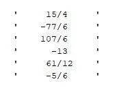
Derivates:

Analytical_derivative =exp(x)*((cos(x)-sin(x))-(cos(x)+(sin(x))));

Forward_differencing =((15/4*cos_x(x))-(77/6*cos_x(x+1*dx))+(107/6*cos_x(x+2*dx))-(13*cos_x(x+3*dx))+(61/12*cos_x(x+4*dx))-(5/6*cos_x(x+5*dx)))/dx^2;

Backward_differencing =((15/4*cos_x(x))-(77/6*cos_x(x-1*dx))+(107/6*cos_x(x-2*dx))-(13*cos_x(x-3*dx))+(61/12*cos_x(x-4*dx))-(5/6*cos_x(x-5*dx)))/dx^2;

Central_differencing =((-1/12*cos_x(x-2*dx))+(4/3*cos_x(x-1*dx))-(5/2*cos_x(x))+(4/3*cos_x(x+1*dx))-(1/12*cos_x(x+2*dx)))/dx^2;

First we have created functions for cos_x, Central difference approximation,Skewed right-sided approximation and Skewed left-sided approximation.

cos_x function:

function [xdot]= cos_x(x)

xdot=(exp(x)*cos(x));

end

1.Central difference approximation function:

function out=centraldiff_approximation(x,dx)

%analytical derivation
%f'(x)=exp(x)*((cos(x)-sin(x))-(cos(x)+(sin(x))));

analytical_derivative =exp(x)*((cos(x)-sin(x))-(cos(x)+(sin(x))));

%numerical derivative

central_differencing =((-1/12*cos_x(x-2*dx))+(4/3*cos_x(x-1*dx))-(5/2*cos_x(x))+(4/3*cos_x(x+1*dx))-(1/12*cos_x(x+2*dx)))/dx^2;

out=abs(central_differencing - analytical_derivative);

end

Skewed right-sided approximation function:

function out=rightskew_approximation(x,dx)

%analytical derivation
%f'(x)=exp(x)*((cos(x)-sin(x))-(cos(x)+(sin(x))));

analytical_derivative =exp(x)*((cos(x)-sin(x))-(cos(x)+(sin(x))));

%numerical derivative

forward_differencing =((15/4*cos_x(x))-(77/6*cos_x(x+1*dx))+(107/6*cos_x(x+2*dx))-(13*cos_x(x+3*dx))+(61/12*cos_x(x+4*dx))-(5/6*cos_x(x+5*dx)))/dx^2;


out=abs(forward_differencing - analytical_derivative);

end

Skewed left-sided approximation function:

function out=leftskew_approximation(x,dx)

%analytical derivation
%f'(x)=exp(x)*((cos(x)-sin(x))-(cos(x)+(sin(x))));

analytical_derivative =exp(x)*((cos(x)-sin(x))-(cos(x)+(sin(x))));

%numerical derivative

backward_differencing =((15/4*cos_x(x))-(77/6*cos_x(x-1*dx))+(107/6*cos_x(x-2*dx))-(13*cos_x(x-3*dx))+(61/12*cos_x(x-4*dx))-(5/6*cos_x(x-5*dx)))/dx^2;


out=abs(backward_differencing - analytical_derivative);

end

After creating functions we should implement this function to main program.

Main program:

clear all 
close all
clc

x=pi/3;

dx =linspace(pi/4,pi/400,20);

for i= 1:length(dx)
    
    rightskew_error(i)=rightskew_approximation(x,dx(i));
    
    leftskew_error(i)=leftskew_approximation(x,dx(i));
    
    centraldiff_error(i)=centraldiff_approximation(x,dx(i));
    
end


loglog(dx,rightskew_error,'g')
hold on
loglog(dx,leftskew_error,'b')
loglog(dx,centraldiff_error,'r')
hold off
xlabel('values of dx')
ylabel('errors')
legend('rightskew','leftskew','centraldiff')

Code explanation:

• Here we are providing x=pi/3 and also we are giving values for dx using linspace command.
• Then,we are creating a loop for the variables schemes of 4th order approximations,to compute the function.
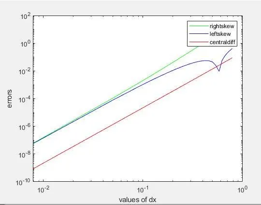
• Then,we are plotting a graph to view the results using loglog command to compare the error values of various schemes of fourth order approximations.

Result:

Conclusion:

As we can see from the above figure the error for the central difference method is very less compared to the skewed methods.

Skewed right and left difference methods almost gives the same results in terms of error for a small value of time step.

Describe why a skewed scheme is useful? What can a skewed scheme do that a CD scheme cannot?

When data from the grid points is only available from either the left or right end i.e. at nodes closer to the boundaries,for computations that requires a high order approximations we make use of skewed schemes.Having a symmetric stencil for computation is not possioble in this scenarios like we do for central differencing schemes or having a low order accuracy.For better consistency of scheme to be maintained the values of dx are kept as low as possible for providing proper computational plots.