Taylor table method and Matlab code

Aim:-

• Derive the 4^th order approximation of the second order derivative using central difference, Skewed right sided difference and Skewed left sided difference.
• Write a program in Matlab to evaluate the second order derivative of the function exp(x)*cos(x).
• Compare analytical results with the derived 3 numerical approximation methods.
• Plot the results of the absolute error for comparison for range of dx.
• Also calculate results using forward difference approximation and backward difference approximations.
• Describe why a skewed scheme is useful? And what can a skewed scheme do that a CD scheme cannot do?
• Write detail report on the above-mention procedure, codes and explain plots and results.

Objective:-

• Firstly, derive 4^th order approximation of the second order derivative by central difference method.
• Same thing derive using skewed right and left side difference method.
• Write codes to calculate analytical expression for the derivative of the function exp(x)*cos(x).
• Write codes to solve same function using above three derived methods using range of dx, to compare approximate results with exact results.
• Next, write program to plot all results in line graph to compare in statistical form.
• Calculate the function using forward difference and backward difference method to compare with error.
• Explain why skewed scheme is useful and significance of skewed scheme over central difference scheme.
• Finally, write detail report explaining all the codes and plots and results of the project.

Discretization:-

In applied mathematics, discretization is the process of transferring continuous function, modes, variable, and equations into discrete counterparts.

In this program we first have to find out exact derivative of the function then we are going to calculate value of the function using first order, second order and fourth order approximation of the function. Finally, we will compare the difference between there errors.

In numerical discretization methos we transfer continuous function, modes, variable, and equation into discrete counterparts so called grid points. The finite difference method is for replacing the partial derivative appearing in governing equations of fluid dynamics, with algebraic difference quotients yielding a system of the algebraic equations which can be solved for the field variable at the specific, discrete grid point in the flow.

Always start program with clear all, close all and clc command to clear all the previous data, close all previously opened figure windows and clc to clear command window.

clear all  % Remove items from workspace, freeing up system memory
close all  % close all the plots and figure window
clc        % clear all data from command window

Provide input value of x and range of dx…

% Given input data
x = pi/3;
dx = linspace(pi/4,pi/400,20);

Analytical Derivative 2^nd order:-

Firstly, lest find out the exact or analytical value of expression by extracting 2^nd order derivative of the function.

To find out 2^nd order derivative of the function exp(x)*cos*(x) in matlab type below codes in command windows.

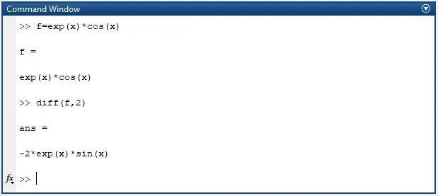
Now, set this expression in main program to latter compare it with other approximations.

% Analytical function = exp(x)*cos(x)
analytical_derivative = -2*exp(x)*sin(x);

Next , we need to apply given function on each grid point using Taylor series so this information we can provide in our approximation methods. So we have range of dx to transfer through all those points, hence, we will use for loop to transfer all the entity in dx array(for length of dx).

for i=1:length(dx)
    
    % Taylor series expansion for required grid points
    a(i) = exp(x-(5*dx(i)))*cos(x-(5*dx(i)));
    b(i) = exp(x-(4*dx(i)))*cos(x-(4*dx(i)));
    c(i) = exp(x-(3*dx(i)))*cos(x-(3*dx(i)));
    d(i) = exp(x-(2*dx(i)))*cos(x-(2*dx(i)));
    e(i) = exp(x-(dx(i)))*cos(x-(dx(i)));
    f(i) = exp(x)*cos(x);
    g(i) = exp(x+(dx(i)))*cos(x+(dx(i)));
    h(i) = exp(x+(2*dx(i)))*cos(x+(2*dx(i)));
    j(i) = exp(x+(3*dx(i)))*cos(x+(3*dx(i)));
    k(i) = exp(x+(4*dx(i)))*cos(x+(4*dx(i)));
    l(i) = exp(x+(5*dx(i)))*cos(x+(5*dx(i)));

Approximation methods to calculate second order derivative.

[1]-Forward Difference method:-

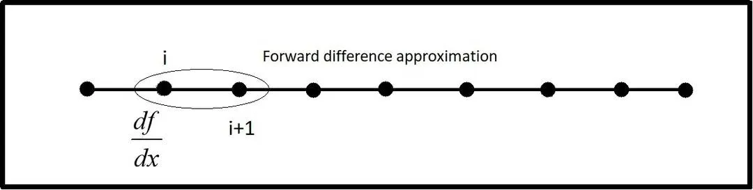
Above calculated analytical expression value of function is our exact value, so, in order to calculate error, we are going to first find out our first order approximation for range of dx by using forward differentiating method. Meaning the derivative is calculated using the information obtain from the point forward(i+1) of the initial point(i).

    % Forward Difference Method
    Forward_Difference(i) = (g(i)-f(i))/(dx(i));

[2]-Backward Difference method:-

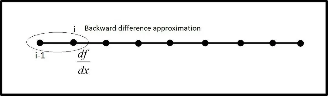
Secondly, we will calculate second order approximation for range of dx using central differentiating method. In this the derivative is calculated using the obtained from the point ahead (i+1) and the point behind (i-1) of the initial point (i).

    % Backward Difference Method
    Backward_Difference(i) = (f(i)-e(i))/(dx(i));

[3]-Central Difference Approximation:-

For central difference scheme,

Number of nodes = Order of derivative + Order of approximations -1

Number of nodes = 2 + 4 -1

:. Number of nodes = 5

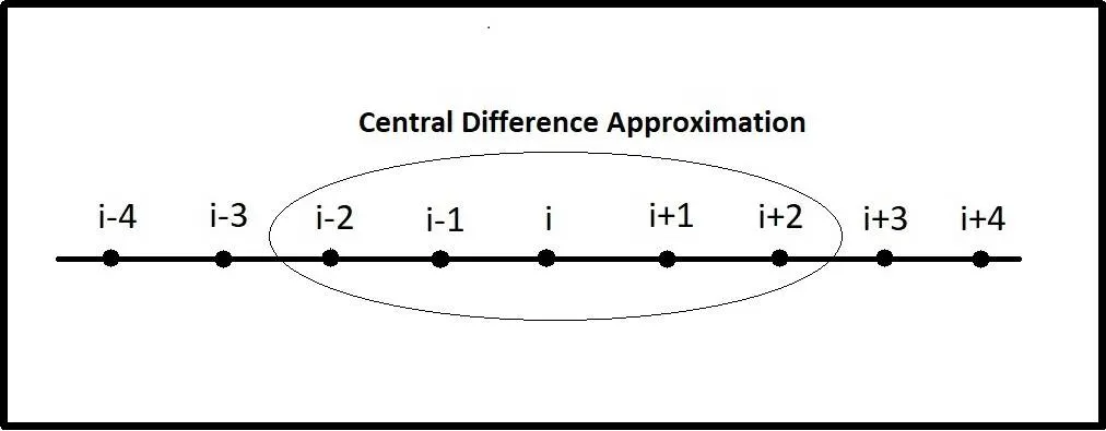
In central difference approximation for 4^th order, the derivative is calculated using the information obtained from the two point ahead (i+2,i+1) and two point behind (i-2,i-1) of initial point(i).

So, 2^nd order derivative, 4^th order accurate central difference scheme equation will be

`Delta x^2 (d^2u)/(dx^2)= af(i-2)+bf(i-1)+cf(i)+df(i+1)+ef(i+2)`

`(d^2u)/(dx^2)= (af(i-2)+bf(i-1)+cf(i)+df(i+1)+ef(i+2))/(Delta x^2)` `…(1)`

	`f(i)`	`f’(i)*Delta(x)`	`f’’(i)*Delta(x)^2`	`f’’’(i)*Delta(x)^3`	`f’’’’(i)*Delta(x)^4`
f(i-2)	a	-2a	4a/2	-8a/6	16a/24
f(i-1)	b	-b	b/2	-b/6	b/24
f(i)	c	0	0	0	0
f(I+1)	d	d	d/2	d/6	d/24
f(I+2)	e	2e	4e/2	8e/6	16e/24
	0	0	1	0	0

Following are the separate Matrices codes for Central Difference method which calculates the value for a, b, c, d, and e.

% Matrices for Central Difference method
A = [1 1 1 1 1;
    -2 -1 0 1 2; 
    4/2 1/2 0 1/2 4/2;
    -8/6 -1/6 0 1/6 8/6;
    16/24 1/24 0 1/24 16/24];
 
B = [0; 0; 1; 0; 0];
 
format rat
C = linsolve(A,B)

Output value of a, b, c, d, and e from above program.

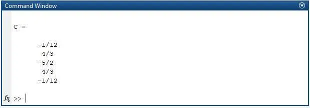
Putting above value in equation number (1) we get

`(d^2u)/(dx^2)= (-f(i-2)+16f(i-1)-30f(i)+16f(i+1)-f(i+2))/(12 Delta x^2)`

Then, put above equation in our codding.

    % Central Difference Method
    Central_Difference(i)=(-1*(d(i))+16*(e(i))-30*(f(i))+16*(g(i))-1*(h(i)))/(12*(dx(i)^2));

[4]-Skewed Right difference Approximation:-

For Skewed difference scheme,

Number of nodes = Order of derivative + Order of approximations

Number of nodes = 2 + 4

:. Number of nodes = 6

:. Skewed Right Difference Schemes are fourth order accurate.

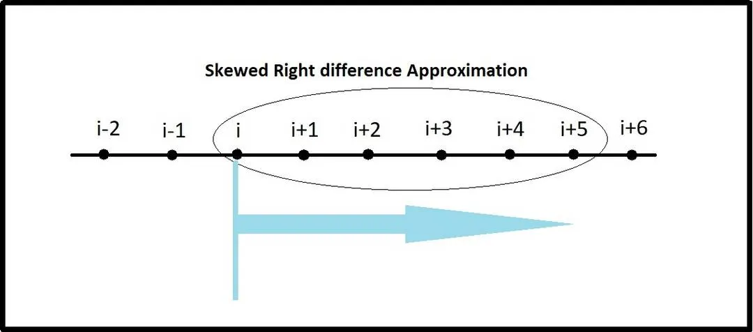
In Skewed right difference approximation method for 4^th order, Approximation is calculated using the information from four point (i+1, i+2, i+3, i+4) ahead from initial point (i).

So, 2^nd order derivative, 4^th order accurate Skewed right difference scheme equation will be

`Delta x^2 (d^2u)/(dx^2)= af(i)+bf(i+1)+cf(i+2)+df(i+3)+ef(i+4)+gf(i+5)`

`(d^2u)/(dx^2)= (af(i)+bf(i+1)+cf(i+2)+df(i+3)+ef(i+4)+gf(i+5))/(Delta x^2)` `…(2)`

	`f(i)`	`f’(i)*Delta(x)`	`f’’(i)*Delta(x)^2`	`f’’’(i)*Delta(x)^3`	`f’’’’(i)*Delta(x)^4`	`f’’’’’(i)*Delta(x)^5`
f(i)	a	0	0	0	0	0
f(i+1)	b	b	b/2	b/6	b/24	b/120
f(i+2)	c	2c	4c/2	8c/6	16c/24	32c/120
f(i+3)	d	3d	9d/2	27d/6	81d/24	243d/120
f(i+4)	e	4e	16e/2	64e/6	25e/24	1024e/120
f(i+5)	f	5f	25f/2	125f/6	625f/24	3125f/120
	0	0	1	0	0	0

Following are the separate Matrices codes for Skewed Right difference approximation method which calculates the value for a, b, c, d, e, and f.

% Matrices for Skewed right side Difference method
A = [1 1 1 1 1 1;
    0 1 2 3 4 5 ; 
    0 1/2 4/2 9/2 16/2 25/2;
    0 1/6 8/6 27/6 64/6 125/6;
    0 1/24 16/24 81/24 256/24 625/24;
    0 1/120 32/120 243/120 1024/120 3125/120];
 
B = [0; 0; 1; 0; 0; 0];
 
format rat
C = linsolve(A,B)

Output value of a, b, c, d, e, and f from above program.

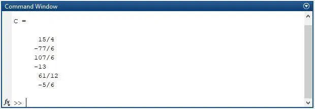
Putting above value in equation number (2) we get

`(d^2u)/(dx^2)= (45f(i)-154f(i+1)+214f(i+2)-156f(i+3)+61f(i+4)-10f(i+5))/(12 Delta x^2)`

Then, put above equation in our codding.

    % Skewed Right sided Difference Method
    Skewed_Right_sided(i)=(45*(f(i))-154*(g(i))+214*(h(i))-156*(j(i))+61*(k(i))-10*(l(i)))/(12*(dx(i))^2);

[5]-Skewed Left difference Approximation:-

For Skewed difference scheme,

Number of nodes = Order of derivative + Order of approximations

Number of nodes = 2 + 4

:. Number of nodes = 6

:. Skewed Left Difference Schemes are fourth order accurate.

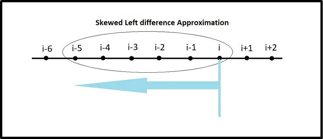
In Skewed left difference approximation method for 4^th order, Approximation is calculated using the information from four point (i-1, i-2, i-3, i-4) behind from initial point (i).

So, 2^nd order derivative, 4^th order accurate Skewed left difference scheme equation will be

`Delta x^2 (d^2u)/(dx^2)= af(i)+bf(i-1)+cf(i-2)+df(i-3)+ef(i-4)+gf(i-5)`

`(d^2u)/(dx^2)= (af(i)+bf(i-1)+cf(i-2)+df(i-3)+ef(i-4)+gf(i-5))/(Delta x^2)` `…(3)`

	`f(i)`	`f’(i)*Delta(x)`	`f’’(i)*Delta(x)^2`	`f’’’(i)*Delta(x)^3`	`f’’’’(i)*Delta(x)^4`	`f’’’’’(i)*Delta(x)^5`
f(i)	a	0	0	0	0	0
f(i-1)	b	-b	b/2	-b/6	b/24	-b/120
f(i-2)	c	-2c	4c/2	-8c/6	16c/24	-32c/120
f(i-3)	d	-3d	9d/2	-27d/6	81d/24	-243d/120
f(i-4)	e	-4e	16e/2	-64e/6	25e/24	-1024e/120
f(i-5)	f	-5f	25f/2	-125f/6	625f/24	-3125f/120
	0	0	1	0	0	0

Following are the separate Matrices codes for Skewed Left difference approximation method which calculates the value for a, b, c, d, e, and f.

% Matrices for Skewed left side Difference method
A = [1 1 1 1 1 1;
    0 -1 -2 -3 -4 -5; 
    0 1/2 4/2 9/2 16/2 25/2;
    0 -1/6 -8/6 -27/6 -64/6 -125/6;
    0 1/24 16/24 81/24 256/24 625/24;
    0 -1/120 -32/120 -243/120 -1024/120 -3125/120];
 
B = [0; 0; 1; 0; 0; 0];
 
format rat
C = linsolve(A,B)

Output value of a, b, c, d, e, and f from above program.

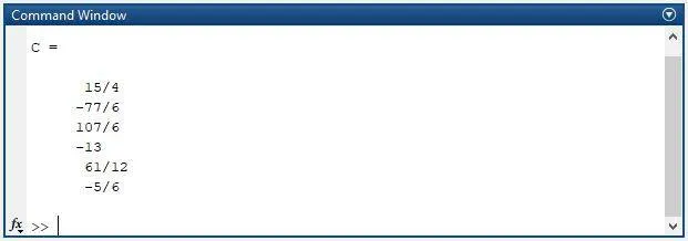
Putting above value in equation number (3) we get

`(d^2u)/(dx^2)= (45f(i)-154f(i-1)+214f(i-2)-156f(i-3)+61f(i-4)-10f(i-5))/(12 Delta x^2)`

Then, put above equation in our codding.

    % Skewed Left sided Difference Method
    Skewed_Left_sided(i)=(45*(f(i))-154*(e(i))+214*(d(i))-156*(c(i))+61*(b(i))-10*(a(i)))/(12*(dx(i))^2);

Error From Approximation

Next, in order to find out error subtract approximate values of all methods from exact or analytical derivative. Afterwards, we will end the for loop.

Error = |Numerical Derivative-Exact derivative|

    % Errors from approximations
    Forward_Difference_error(i) = abs(Forward_Difference(i)-analytical_derivative);
    Backward_Difference_error(i)= abs(Backward_Difference(i)-analytical_derivative);
    Central_Difference_error(i) = abs(Central_Difference(i)-analytical_derivative);
    Skewed_Right_sided_error(i) = abs(Skewed_Right_sided(i)-analytical_derivative);
    Skewed_Left_sided_error(i)  = abs(Skewed_Left_sided(i)-analytical_derivative);
    
end

Furthermore, we have to plot the graph from above data. We will use following codes to plot line graph.

figure(1)
set(gcf, 'Position',  [10, 50, 900, 900])    % set the size of figure window
loglog(dx,Forward_Difference_error,'k','linewidth',1,'marker','square')
hold on
loglog(dx,Backward_Difference_error,'m','linewidth',1,'marker','pentagram')
loglog(dx,Central_Difference_error,'r','linewidth',1,'marker','hexagram')
loglog(dx,Skewed_Right_sided_error,'b','linewidth',1,'marker','o')
loglog(dx,Skewed_Left_sided_error,'g','linewidth',1,'marker','square')
hold off
legend({'Forward Difference approximations','Backward Difference approximations','Central Difference approximations','Skewed Right sided Difference approximations','Skewed Left sided Difference approximations'},'location','southeast','fontsize',12,'fontweight','bold')
title({'Comparison of Errors for various Finite';'Difference approximations'},'fontsize',20,'fontweight','bold')
xlabel('<-----     Range of dx     ----->','fontsize',14,'fontweight','bold')
ylabel('<-----     Absolute Error     ----->','fontsize',14,'fontweight','bold')
grid on

Output for above codes:-

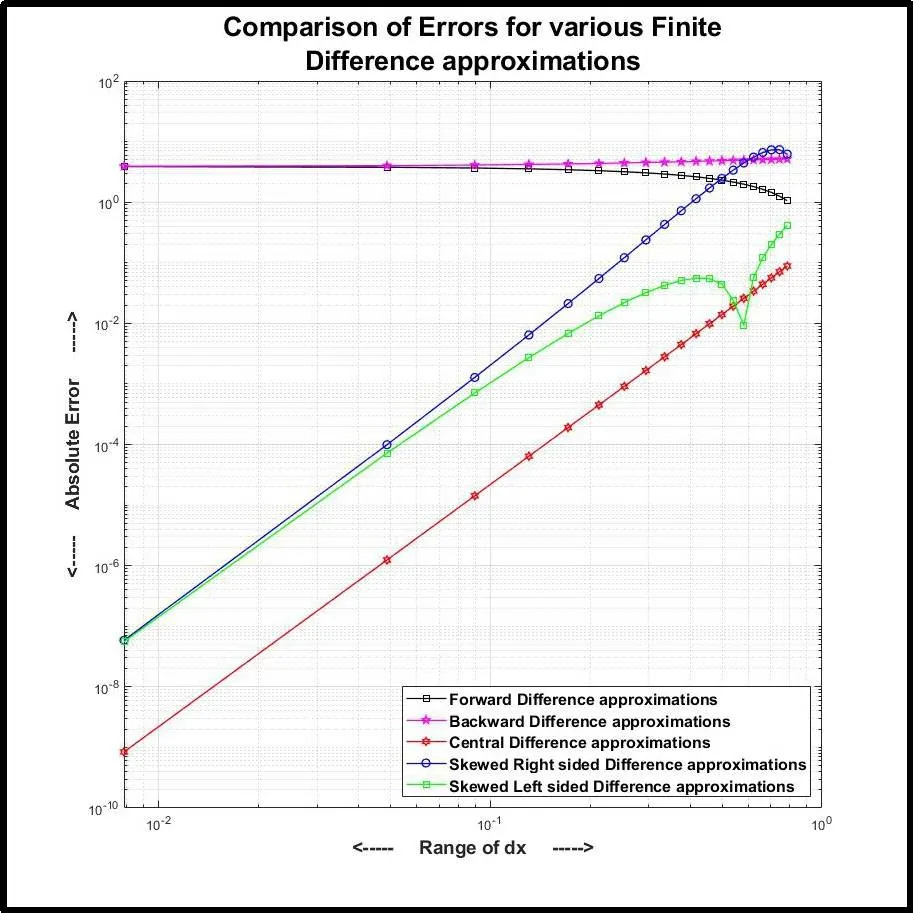
Graph exhibits the results of amount of absolute error from Froward Difference approximations, Backward difference approximations, Central difference approximations, Skewed right side Difference approximations and Skewed left side difference approximations in given range of dx.

A brief overview of plot portray some intriguing pattern in which Central difference scheme is showing more less error than any other method. Slope of Skewed Right side approximation curve is almost parallel to the central difference method curve, on the other hand, the slope of Skewed left scheme curve is at staring showing a extreme downward variation but later its giving same absolute error as Skewed right scheme.

If we take closer look at Forward and backward difference approximations there error is far more higher than other three method’s curve because they have first order approximations.

Overall, Central Difference method is giving the best results but then the question arises “why a Skewed scheme is useful?” and ” What can a skewed scheme do that a CD scheme cannot?”

Why a Skewed scheme is useful? and What can a skewed scheme do that a CD scheme cannot?

Firstly, if we talk about central difference method it required information from both side of the initial point, so, in case, we have initial point completely one, either left or right, side of the grid which do not have nodes on the other side. In this condition, we have to apply Taylor approximation using skewed scheme - serially - either on the negative or positive direction where nodes are present.

In such problems, where we cannot employ central difference method to get our required result, as information is not provided in the both direction, therefor, we prefer skewed left or right scheme to compute the results. Detail example is we had seen in this project to understand this concept

In order to compare slope of error line from all the approximation schemes, first, find out slope between each point. It will give us data in arrays form.

% Slope of each scheme error
Slope_Forward_Difference = gradient(log10(Forward_Difference_error),log10(dx))
Slope_Backward_Difference = gradient(log10(Backward_Difference_error),log10(dx)); 
Slope_Central_Difference = gradient(log10(Central_Difference_error),log10(dx)); 
Slope_Skewed_Right_sided = gradient(log10(Skewed_Right_sided_error),log10(dx)); 
Slope_Skewed_Left_sided = gradient(log10(Skewed_Left_sided_error),log10(dx)); 

Use following codes to plot the slope data for each approximation method.

figure(2)
set(gcf,'position',[10 50 900 900])
plot(Slope_Forward_Difference,'k','linewidth',1,'marker','square')
hold on
plot(Slope_Backward_Difference,'m','linewidth',1,'marker','pentagram')
plot(Slope_Central_Difference,'r','linewidth',1,'marker','hexagram')
plot(Slope_Skewed_Right_sided,'b','linewidth',1,'marker','o')
plot(Slope_Skewed_Left_sided,'g','linewidth',1,'marker','square')
title('Slope for each approximations to minimize Error','fontsize',20,'fontweight','bold')
xlabel('Number of points in range of dx   ----->','fontsize',14,'fontweight','bold')
ylabel('<------     Slope of curve    ----->','fontsize',14,'fontweight','bold')
legend({'Slope for Forward Difference','Slope for Backward Difference','Slope for Central Difference','Slope for Skewed Right sided','Slope for Skewed Right sided'},'location','southeast','fontsize',12,'fontweight','bold')
grid on 
hold off

Output for above codes:-

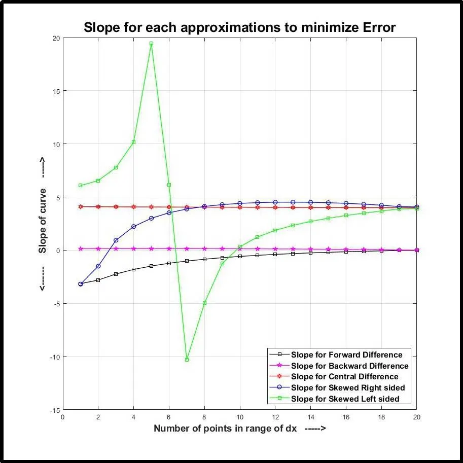
From above plot we get the data of slope of curve we to minimize the absolute error from respective approximation method for the rang of dx.

A glimpse over the graph illustrates some intriguing patterns in which slope of Skewed right and left scheme curve and central difference approximation curve at the initial level are different but at the end its almost constant.

Same way if we talk about Forward and backward methods curves, their slope value is lower than other three. And the skewed left side scheme have higher value of slope among all others even after central difference method is the most accurate method among other four schemes.

Conclusion

• Study about different approximation methods to get results in with various required accuracy.
• Understood Taylor table method to evaluate value of approximation.
• Learned when to use skewed scheme and why it is important over Central difference approximations.
• Cleared all the concept for how to find number of nodes to consider for specific order of approximations in Central difference and skewed scheme.

Complete Program:-

clear all  % Remove items from workspace, freeing up system memory
close all  % close all the plots and figure window
clc        % clear all data from command window

% Given input data
x = pi/3;
dx = linspace(pi/4,pi/400,20)

% Analytical function = exp(x)*cos(x)
analytical_derivative = -2*exp(x)*sin(x);

for i=1:length(dx)
    
    % Taylor series expansion for required grid points
    a(i) = exp(x-(5*dx(i)))*cos(x-(5*dx(i)));
    b(i) = exp(x-(4*dx(i)))*cos(x-(4*dx(i)));
    c(i) = exp(x-(3*dx(i)))*cos(x-(3*dx(i)));
    d(i) = exp(x-(2*dx(i)))*cos(x-(2*dx(i)));
    e(i) = exp(x-(dx(i)))*cos(x-(dx(i)));
    f(i) = exp(x)*cos(x);
    g(i) = exp(x+(dx(i)))*cos(x+(dx(i)));
    h(i) = exp(x+(2*dx(i)))*cos(x+(2*dx(i)));
    j(i) = exp(x+(3*dx(i)))*cos(x+(3*dx(i)));
    k(i) = exp(x+(4*dx(i)))*cos(x+(4*dx(i)));
    l(i) = exp(x+(5*dx(i)))*cos(x+(5*dx(i)));
    
    % Forward Difference Method
    Forward_Difference(i) = (g(i)-f(i))/(dx(i));
    
    % Backward Difference Method
    Backward_Difference(i) = (f(i)-e(i))/(dx(i));
   
    % Central Difference Method
    Central_Difference(i)=(-1*(d(i))+16*(e(i))-30*(f(i))+16*(g(i))-1*(h(i)))/(12*(dx(i)^2));
    
    % Skewed Right sided Difference Method
    Skewed_Right_sided(i)=(45*(f(i))-154*(g(i))+214*(h(i))-156*(j(i))+61*(k(i))-10*(l(i)))/(12*(dx(i))^2);
    
    % Skewed Left sided Difference Method
    Skewed_Left_sided(i)=(45*(f(i))-154*(e(i))+214*(d(i))-156*(c(i))+61*(b(i))-10*(a(i)))/(12*(dx(i))^2);
    
    % Errors from approximations
    Forward_Difference_error(i) = abs(Forward_Difference(i)-analytical_derivative);
    Backward_Difference_error(i)= abs(Backward_Difference(i)-analytical_derivative);
    Central_Difference_error(i) = abs(Central_Difference(i)-analytical_derivative);
    Skewed_Right_sided_error(i) = abs(Skewed_Right_sided(i)-analytical_derivative);
    Skewed_Left_sided_error(i)  = abs(Skewed_Left_sided(i)-analytical_derivative);
    
end

figure(1)
set(gcf, 'Position',  [10, 50, 900, 900])    % set the size of figure window
loglog(dx,Forward_Difference_error,'k','linewidth',1,'marker','square')
hold on
loglog(dx,Backward_Difference_error,'m','linewidth',1,'marker','pentagram')
loglog(dx,Central_Difference_error,'r','linewidth',1,'marker','hexagram')
loglog(dx,Skewed_Right_sided_error,'b','linewidth',1,'marker','o')
loglog(dx,Skewed_Left_sided_error,'g','linewidth',1,'marker','square')
hold off
legend({'Forward Difference approximations','Backward Difference approximations','Central Difference approximations','Skewed Right sided Difference approximations','Skewed Left sided Difference approximations'},'location','southeast','fontsize',12,'fontweight','bold')
title({'Comparison of Errors for various Finite';'Difference approximations'},'fontsize',20,'fontweight','bold')
xlabel('<-----     Range of dx     ----->','fontsize',14,'fontweight','bold')
ylabel('<-----     Absolute Error     ----->','fontsize',14,'fontweight','bold')
grid on

% Slope of each scheme error
Slope_Forward_Difference = gradient(log10(Forward_Difference_error),log10(dx))
Slope_Backward_Difference = gradient(log10(Backward_Difference_error),log10(dx)); 
Slope_Central_Difference = gradient(log10(Central_Difference_error),log10(dx)); 
Slope_Skewed_Right_sided = gradient(log10(Skewed_Right_sided_error),log10(dx)); 
Slope_Skewed_Left_sided = gradient(log10(Skewed_Left_sided_error),log10(dx)); 

figure(2)
set(gcf,'position',[10 50 900 900])
plot(Slope_Forward_Difference,'k','linewidth',1,'marker','square')
hold on
plot(Slope_Backward_Difference,'m','linewidth',1,'marker','pentagram')
plot(Slope_Central_Difference,'r','linewidth',1,'marker','hexagram')
plot(Slope_Skewed_Right_sided,'b','linewidth',1,'marker','o')
plot(Slope_Skewed_Left_sided,'g','linewidth',1,'marker','square')
title('Slope for each approximations to minimize Error','fontsize',20,'fontweight','bold')
xlabel('Number of points in range of dx   ----->','fontsize',14,'fontweight','bold')
ylabel('<------     Slope of curve    ----->','fontsize',14,'fontweight','bold')
legend({'Slope for Forward Difference','Slope for Backward Difference','Slope for Central Difference','Slope for Skewed Right sided','Slope for Skewed Left sided'},'location','southeast','fontsize',12,'fontweight','bold')
grid on 
hold off