Week 3 - Solving second order ODEs
Solving second order ODEs
In Engineering, ODE is used to describe the transient behavior of a system. A simple example is a pendulum. The way the pendulum moves depends on Newton's second law. When this law is written down, we get a second-order Ordinary Differential Equation that describes the position of the "ball" w.r.t time.
Similarly, there are hundreds of ODEs that describe key phenomena and if WE have the ability to solve these equations then we will be able to simulate any of these systems.
Aim:
- To write a program that solves the following ODE.
- Animate the motion of the pendulum.
Given:
This ODE represents the equation of motion of a simple pendulum with damping
In the above equation:
`(d^2theta)/(dt^2)+ (b/m)((d theta)/dt)+ (g/l)sin theta =0`
where,
g = gravity in m/s2,
L = length of the pendulum in m,
m = mass of the ball in kg,
b=damping coefficient.
To write a program in Python that will simulate the pendulum motion
use,
L=1 meter,
m=1 kg,
b=0.05.
g=9.81 m/s2.
We have to simulate the motion between 0-20 sec, for angular displacement=0,angular velocity=3 rad/sec at time t=0.
When we will do this, will get the position of the pendulum as a function of time. Use this information to animate the motion of the pendulum, as shown in the below figure.
Procedure:
- Import all the required library files.
- Define a function named Model and pass several input arguments theta,t,b,g,l,m.
- Here the theta1_dt and theta2_dt are the derivatives in which the theta1 and theta2 are the angular displacement and velocity.
- dtheta_dt carries the velocity and angular acceleration.
- Give input and initial condition and time for oscillation. The initial condition has to be given for both ODEs so it is 0 and 3. The first ODE is the displacement and the second is Velocity(0).
- Odeint command is in the scipy module, so make sure to import scipy before using it.
- It is a function that integrates ODE or the system of ODE.
- Model is a function that represents the ODE system(dtheta_dt1 and dtheta_dt2) and it has to be defined.
- Now we have to plot them.
Main Code:
import math
import numpy as np
import matplotlib.pyplot as plt
from scipy.integrate import odeint

def Model(theta,t,b,g,l,m):
	theta1=theta[0] # displacement
	theta2=theta[1] # velocity
	dthetal_dt= theta2 # ODE 1
	dtheta2_dt= -(b/m)*theta2-(g/1) * math.sin(theta1) # ODE 2
	dtheta_dt=[dthetal_dt, dtheta2_dt] # PUT BOTH ODE IN SINGLE ODE.
	return dtheta_dt

# inputs
b=0.05
g=9.81
l=1
m=0.1
# initial condition
theta_0= [0,3]

# time
t= np.linspace(0,20,350)

# solve ODE
theta = odeint(Model, theta_0,t, args = (b,g,l,m))

#plot results
plt.plot(t,theta[:,0],'b-', label= r'$\frac{d\theta_1}{dt}=\theta2$') # time vs displacement(1st column of theta)
plt.plot(t,theta[:,1],'g--', label= r'$\frac{d\theta_1}{dt}= -\frac{b}{m}\theta_2-\frac{g}{L}sin\theta_1$') # time vs velocity(2nd column of theta)
plt.ylabel('Plot')
plt.xlabel('time')
plt.legend(loc='best')
plt.show()

#initial condition
x0=0
y0=0
ct=1
for ang_disp in theta[:,0]:  # for value of anguler displacement in theta for all rows of 1st column.

	x1= l * math.sin(ang_disp)
	y1=-( l * math.cos(ang_disp))


	FileName = 'ODE%04d.png' % ct
	ct = ct+1
	plt.figure()
	plt.plot([-1,1],[0,0], "black",linewidth = 3) # horizontal support
	plt.plot([x0,x1],[y0,y1],"blue") # string conncted with points
	plt.plot(x1,y1,'-o', markersize=10) # pendulam representation
	plt.xlim([-2.5,2.5])
	plt.ylim([-2.5,2.5])
	plt.savefig(FileName)
Results:
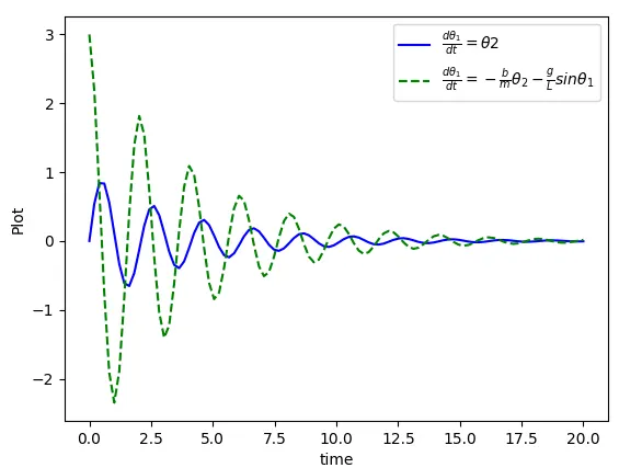
Due to the damping, this converges towards the end.
Link: