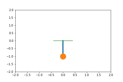
Solving second order ODEs using PYTHON

SOLVING SECOND ORDER DIFFRENTIAL EQUATION IN PYTHON

PROBLEM STATEMENT–

The aim of this project was to write a program in PYTHON that solves the given ODE is used to describe the transient behaviour of a pendulum. The provided equation is the equation for damping of the oscillating bob or ball, which is attached to a fixed length of string.

The initial displacement and of 0m and 3 m/s respectively are provided to initialise the oscillation. Further, a fixed time of 20 sec is to be observed to study the effect of damping.

The length of string and mass of bob is considered to be unity. Acceleration due to gravity is provided and the damping coefficient is considered as 0.05.

OBJECTIVES OF THE PROJECT-

• To solve the 2^nd order ODEs.
• To plot graphs of ‘angular displacement vs time’ and ‘angular velocity vs time’
• To produce an animation.

GOVERNING EQUATION-

The governing equation for the damping effect of the pendulum is given a second order differential equation

The governing equation is the basic equation for the motion of a simple pendulum with damping

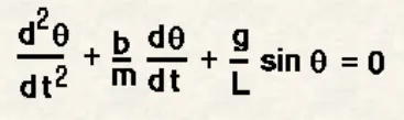
Where,

THETA- angle suspended by string with respect to the string axis passing through mean

position of bob

b - damping coefficient

m - mass of bob

g - acceleration due to gravity

l - length of string to which bob is attached.

BODY OF THE CONTENT:

Damping is the process of dissipation of energy in an oscillating or vibrating body. There are different kinds of damping: -

1. Viscous damping- due to medium
2. Dry friction damping- due to friction between surfaces due to lack of lubrication
3. Hysteretic damping- due to friction between planes by slips or slide as the material deforms
4. Magnetic damping- due to magnetic effect

The pendulum's movement depends on the Newton’s second law. This law is written as a second order Ordinary Differential Equation that describes the position of the "ball" with respect to time. The ball is provided with an initial velocity at zero displacement and allowed to oscillate. It slowly gets damped under the effect of medium and gravity as the equation denotes it.

For python, solving higher order ODE is not possible directly. So the higher order ODE is to be broken into twodifferential equations of order 1. This is done by the following steps:

Initially, the provided angle theta is assumed to be equal to a new variable that is ‘theta1’. This ‘theta1’ is differentiated with respect to time and the result{d(theta1)/dt} is equal to ‘theta2’. When we differentiate theta2 with respect to time, we get {d(theta2)/dt }which is exactly the first term of damping equation but in first order.

• Theta = theta 1
• d(theta1)/dt = theta2
• d(theta2)/dt = d(d(theta1)/dt)/dt = d(d(Theta)/dt)/dt = d^2(Theta)/ (dt)^2

Substituting the equations with the damping equation, we get the two equations for 2^nd order ODE, as follows

1. d(theta1)/dt = theta2
2. d(theta2)/dt= -{(b/m) *theta2}-{(g/l) *sin(theta1)}

Now these two first order ODE will be solved using the inbuilt solver in Python. For this a library named “scipy.intergrate”, a solver “odeint” is imported. This is a older solver for integrating a system of ODEs using Isoda. It was implemented as solver in FORTRAN (mostly ODEPACK).

import math
import matplotlib.pyplot as plt
import numpy as nm
from scipy.integrate import odeint
import imageio
import os

#creating first order ODEs
def model(theta,t,b,g,l,m):
    theta1 = theta[0]
    theta2 = theta[1]
    dtheta1_dt = theta2                                    #first order ODE-1
    dtheta2_dt = -(b/m)*theta2 - (g/l)*math.sin(theta1)    #first order ODE-2
    dtheta_dt = [dtheta1_dt,dtheta2_dt]       #combining results as a function of theta
    return dtheta_dt

#given values
b = 0.05
g = 9.81
l = 1
m = 1

#initial condition
theta_0 = [0,3]

#time points
t = nm.linspace(0,20,200)

#solving ode
theta = odeint(model,theta_0,t,args = (b,g,l,m))

#results
plt.plot(t,theta[:,0],'b-')           #displacement graph
plt.plot(t,theta[:,1],'r--',)         #velocity graph
plt.xlabel("time")
plt.ylabel("plot")
plt.show()

thetaRes = theta[:,0]                #array with displacement
ct=1                                 #counter
for t in thetaRes:
    
    x1=0                             #initial point coordinates
    y1=0               
    
    x2=l*math.sin(t)                 #unfixed end of string's point coordinates
    y2=-l*math.cos(t)
    
    filename = '%03d.png' % ct
    ct=ct+1                          #increment to counter
    
    plt.figure()
    plt.plot([x1,x2],[y1,y2],linewidth =4)                  #the string
    plt.plot(x2,y2,'o',markersize =20)                      #ball
    plt.plot([-0.4,0.4],[0,y1])               #the fixed base for swinging pendulum
    plt.xlim(-1.5,1.5)
    plt.ylim(-1.5,1.5)
    
    plt.savefig(filename)
    
#making the animation

files = os.listdir('gif')                     #listing the directory

image_path = [os.path.join('gif',file)for file in files] #compiling png files

gif = []
for img in image_path:                           #reading the png files
    gif.append(imageio.imread(img))
    
imageio.mimwrite('rob_arm.gif',gif,fps = 12)     #making animation

Let us see the code,

First, the libraries and solver were imported. These contains the basic commands which will be applied throughout the code.

• Math – deals with mathematical commands such as pi, trigonometric functions etc
• pyplot – this module has plotting commands from matlab which makes representation easy
• Numpy - numpy consists of functions from C and FORTRAN to ease computation
• Scipy – it consists of functions for calculus
• Imageio – this lib will help us create the gif
• Os – this module helps us to interact with operating system.

Now the function “model” is defined in which the theta1 and theta2 along with the first order ODEs will be defined. The values will be returned to the capture all the values rather than just the last one.

dtheta_dt = [dtheta1_dt, dtheta2_dt] this row combines the two first order ODEs

The following will provide value from the previous iteration when the function will be called to be solved.

• theta1 = theta[0]
• theta2 = theta[1]

various input parameters are provided as per the problem statement and for time, linspace is used for fixed number of intervals. The library numpy is used to use linspace as it is not an inbuilt function in python. For initial condition, displacement and velocity as been defined in single array.

The odeint solver is executed as per format.

theta = odeint(model,theta_0,t,args = (b,g,l,m))

here, model is the function to be solved with initial condition “theta_0” and for the time array of “t”. The constants used in the process is present as “args = (b,g,l,m)”.

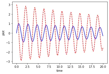
Plots were plotted using matplotlib.pyplot module. One plot for displacement and velocity was plotted such that displacement was in blue colour straight line and velocity graph was in red colour dotted line(fig.results1).

For the animation, frames were created using a for loop with displacement array “thetaRes”. In the for loop, one point(x1,y1) was kept constant and other moved according to the displacement result. To name the file, command was used and to capture every new plot, a counter was introduced. Further, the required plots were provided using matplotlib.pyplot module. Now the frames are saved using “plt.savefig(filename)”. All the frames were transferred to a new folder named gif. This folder will be used to make animation.

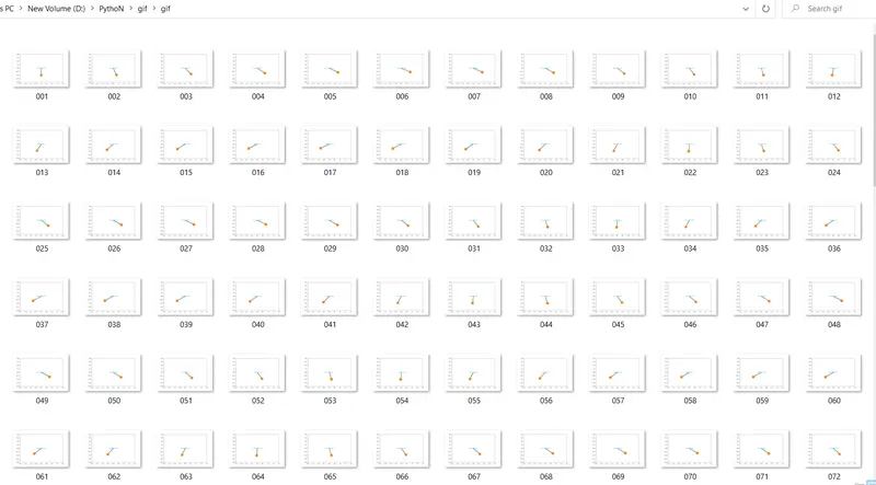
The last process consists of producing animation. For this imageio was used. The first step consists of list files in the saved directory. Further, all the files are made available to be joined. After this a for loop is made to read all the compiled files in gif folder to be made into animation. Finally “imageio.mimwrite” command was used to make the animation with a name, file type(“gif”) and frames per second.

RESULTS-

The plot for displacement and velocity graph against time is plotted and is shown below. The damping effect can be seen as the maxima and minima of oscillation decreases as the time proceeds. Similar trend is seen in displacement. The validation of graph can be done by looking at initial point of velocity (3m/s) and displacement as (0m).

• Blue - Displacement vs time
• Dotted Red - Velocity vs time

The produced gif for animation is provided below. The damping is relevant as the extreme point decreases with time.