Study of Air Standard Cycle using MATLAB

1.AIM:

To solve an Otto cycle using Matlab

2.GOVERNING EQUATIONS:

Ideal gas equation PV = mRT

Isentropic Equation PV^γ =C

Swept volume v_s = pi/4*bore^2*stroke

Clearance volume v_c = v_s/(cr-1)

Total volume v_t = v_s + v_c

Volume at particular cranck angle -

V= (1 + 0.5(cr- 1)((R + 1-cos(θ)) - ((R^2 - sin(θ)^2)^0.5))).*v_c

(R- engine rod ratio θ=crank angle cr- compression ratio)

Thermal efficiency E= 1- ((T4-T1)/(T3-T2))

3.OBJECTIVES OF THE PROJECT:

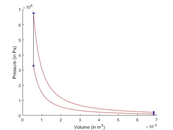
• PV diagram of the Otto cycle
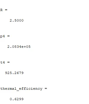
• Calculate Thermal Efficiency of the cycle

4.BODY OF THE CONTENT:

The Otto cycle is a thermodynamic cycle which consists of processes in spark ignition engine. The process starts from BDC with air fuel intake. It consists of the following processes-

1. Isentropic compression
2. Constant volume heat addition (spark ignition)
3. Isentropic expansion
4. Constant volume heat rejection (exhaust)

The process starts from pont 1 where the piston is at BDC and moves towards TDC. The air fuel compression takes place and the starting of process 2-3, the spark is generated to produce power. As a result pressure increases at constant volume. Due to this the process 3-4 takes place which is the power stroke. In this power is transmitted and piston moves from TDC to BDC again. The exhaust stroke is 4-1 when heat is released and gas is exhausted through exhaust port. The process continues. The typical firing order of Inline four cylinder engine is 1-3-4-2.

The provided parameters were Pressure and Temperature (1) at end of start of cycle and along with the temperature at the start of end of process 2. The further details consist of bore diameter, stroke length, connecting rod length, compression ratio (cr) and ‘γ’ (Cp/Cv). The aim was to calculate all the parameters in order to form PV diagram and find thermal efficiency of the cycle.

For calculation of volume at process 1 and 2, clearance and swept volume were calculated using the formulae given above. Hence and

From ideal gas equation, was calculated.

For process 3, , pressure was calculated by ideal gas equation.

For process 4, , pressure was calculated by isentropic equation and temperature was calculated using the ideal gas equation.

For the continuity of the isentropic processes, a function was created. The formula used, gives values of volume at specific values of crank angles. Linspace command is used to randomise the values of crank angle. Here calling for the function is done with input parameters as bore, stroke, connecting rod length, starting angle of crank and ending angle of crank.

note : the name of the function does not denote relation with function. It is just for name sake.

function[volume]= air_ratio(bore,stroke,con_rod,comr,st_angle,end_angle)

R= (2*con_rod)/(stroke)

v_s= pi/4*stroke*bore^2;
v_c= v_s/(comr-1);

theta= linspace(st_angle,end_angle,30);

term1= 0.5*(comr- 1);
term2= R + 1-cosd(theta);
term3= (R^2 - sind(theta).^2).^0.5;

volume = (1 + term1.*(term2 - term3)).*v_c



end

For compression (process1), crank angle varies from 180deg to 0deg i.e. from BDC to TDC

For expansion (process 2), crank angle varies from 0deg to 180deg ie from TDC to BDC.

the commands vol_comp and pres_comp are for compression cycle in which calling of function 'air_ratio'

the commands vol_exp and pres_exp are for expansion cycle in which calling of function 'air_ratio'

clear all
close all
clc

%engine discription and constants
bore = 0.2
stroke = 0.2
c_rod = 0.25
cr=12
gamma = 1.4

%engine parameters
p1 = 101325
t1 = 450
t3 = 2500

%swept and clearance volume
v_s = pi/4*bore^2*stroke
v_c = v_s/(cr-1)

v1 = v_c + v_s
v2 = v_c 

p2 = p1*(v1/v2)^gamma
t2 = (p2*v2)/(p1*v1/t1)

vol_comp  = air_ratio(bore,stroke,c_rod,cr,180,0)
pres_comp = (p1*v1^gamma)./vol_comp.^gamma

v3=v2

p3= p2*(t3/t2)

vol_exp  = air_ratio(bore,stroke,c_rod,cr,180,360)
pres_exp = (p3*v3^gamma)./vol_exp.^gamma

v4 = v1

p4= p3*(v3/v4)^gamma

t4= t1*(p4/p1)

%thermal efficiency
thermal_efficiency = 1- ((t4-t1)/(t3-t2))

hold on
plot(v1,p1,'*','color','b')
plot(v2,p2,'*','color','b')
plot(v3,p3,'*','color','b')
plot(v4,p4,'*','color','b')
plot(vol_comp,pres_comp,'color','r')
plot(vol_exp,pres_exp,'color','r')
plot([v2 v3],[p2 p3],'color','black')
plot([v4 v1],[p4 p1],'color','black')
xlabel('Volume (in m^3)')
ylabel('Pressure (in Pa)')

Thermal efficiency of the process was calculated by the formula.

The PV graph was plotted by 'plot' command with xlabel for x axis naming as Volume and ylabel for y axis labeling as Pressure and is shown as

the efficiency and other output of codes are as follows.

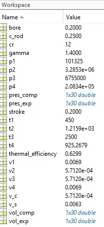
The validity of the code can be checked by increase in values of pressure at process 2 and 3 and decrease at 4 and 1.

CONCLUSION -

• The exact trace of an otto cycle with given parameters has been plotted using Matlab.
• The process of Icentropic expansion and compression were traced by calling a predefined function.
• The counter checking has been done by taking the ideal graph as reference and also by checking increment and decrement in pressure at different process points.
• The thermal efficiency was calculated.