Week 3 - Solving second order ODEs

Aim:

To simulate the transient behaviour of a simple pendulum using Python.

Objective:

• To solve the following ODE and simulate the transient behaviour of a simple pendulum.

`d^2theta//dt^2+(b/m)d theta//dt+(g/l)sin theta =0`

• To make an animation of the transient behaviour.

Theory:

Simple Pendulum:

A Simple Pendulum is a simple arrangement of a string fixed at one end and a bob making to-fro motion at the other end.This transient beahviour is governed by a Second-order Ordinary Differential Equation(ODE).The equation is as follows,

`d^2theta//dt^2+(b/m)d theta//dt+(g/l)sin theta =0`

Where,

b is theDamping coefficient,

m is the mass of the bob(kg),

g is the gravitational force(m/s^2),

l is the length of the string(m).

Damping Coefficient:

Damping Coefficient is a material property which gives the ability of a material to release energy.

Description of Program:

1)The inputs and the initial conditions are given.

2)The second order ODE is simplified to two single order ODE.

3)A function is written to solve these two single order ODEs.

4)This function is then called into the main program.

5)This gives the behaviour of the bob with respect to time.

6)A for loop is created and the simulation of the bob is created using the displacement.

7)A movie is created using the the Image magick application.

Program:

# Simple Pendulum

import math
import matplotlib.pyplot as plt 
import numpy as np 
from scipy.integrate import odeint

# Defining Fuction:
def xyz(theta,time,l,m,b,g):
	 theta_1 = theta[0]
	 theta_2 = theta[1]

	 dtheta1_dt = theta_2
	 dtheta2_dt = -((b/m)*theta_2) - (g/l)*math.sin(theta_1)
	 dtheta_dt = [dtheta1_dt, dtheta2_dt]
	 return dtheta_dt

#Inputs
l = 1
m = 1
b = 0.5
g = 9.81

#Initial Condotion:
theta = [0,3]

#time condition:
time = np.linspace(0,20,100)

#Calling Function
t = odeint(xyz,theta,time,args = (l,m,b,g))

plt.plot(time,t[:,0],'b-', label = r'Displacement(m)')
plt.plot(time,t[:,1],'r--', label = r'Velocity(m/s)')
plt.xlabel('Time(sec)')
plt.ylabel('Magnitude')
plt.ylim(-4,4)
plt.legend()
plt.show()

#Plotting the Simple pendulum positions:
a = t[:,0]
ct = 1
for i in a:
	x1 = 0
	y1 = 0

	x2 = l*math.sin(i)
	y2 = -(l*math.cos(i))
	
	filename = 'pic%03d.png' %ct
	ct = ct+1
	plt.figure()
	plt.plot([0,x2],[0,y2])
	plt.plot([x1,x2],[y1,y2],'o')
	plt.xlim(-2,2)
	plt.ylim(-2,2)
	plt.savefig(filename)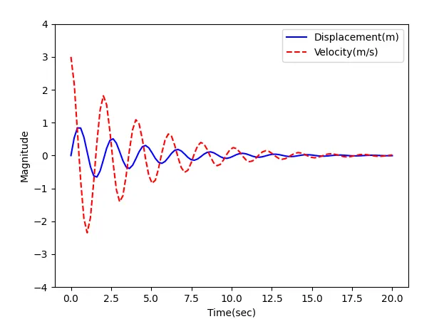

Link of the Simple Pendulum Gif:

https://drive.google.com/file/d/1cvbUPXWu9vqS_7JcOcKyLe3V6i563Xgw/view?usp=sharing

Result and Conclusion:

• The transient behaviour of the Simple Pendulum was tracked by solving the Second-order ODE which showed that the veloicty got damped after a certain point which resulted the pendulum to stand still.
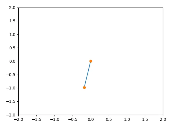
• An animation was created of the transient behaviour.