Week 3 - Solving second order ODEs
Solving the second order ODEs of Simple Pendulum using Matlab
Introduction: A simple pendulum is an oscillating device consisting of point mass suspended from a spring or rod of negligible mass.
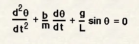
Differential equation governing the oscialltion of a simple pendulum considering a spring-mass-damper system is:
%Main program code
Clear all %clears workspace
close all %closes all the figures generated
clc %clears command window
%Input parameters
b=0.04; %damping coefficient
g=9.81 %acceleration due to gravity in m/s2
l=1 %length of the rod in m
m=0.1; %mass of the pendulum in kg
ct=1 %counter variable
x0=0 %x-xordinate of pendulum origin/pivot point
y0=0 %y-xordinate of pendulum origin/pivot point
%initial conditions
theta_0=[0;3]; %o is the initial angular displacement and 3 is the initial velocity
%time limit
t_span=linspace(0,20,500);
%solving the ODE
[t,results]=ode45(@(t,theta)ode_func(t,theta,b,g,l,m),t_span,theta_0);
%plotting
figure(1)
plot(t,results(:,1)) %In the result matrix, first column is angular displacement
hold on
plot(t,results(:,2)) %In the result matrix, second column is the velocity
xlabel('Time in seconds');
ylabel('Displacement and velocity');
legend('Displacement','Velocity');
%creating animation
for i=1:length(results(:,2))
figure(2)
x1=l*sin(results(i,1));
y1=-(l*cos(results(i,1)));
plot([-1.5 1.5],[0 0],'linewidth',3,'color',[0.54 0.42 0.52]) %Fixed support shown as a line
axis([-1 1 -1.5 1])
hold on
line([x0 x1],[y0 y1],'linewidth',5,'color','b'); %pendulum rod which will change its position %instantaneously w.r.t time
plot(x1,y1,'o','markersize',15,'markerfacecolor','r'); %Pendulum bob which is fixed to the rod.
M(ct)=getframe(gcf);
ct=ct+1;
hold off
end
%create movie
movie(M);
videofile=VideoWriter('SimplePendulum_oscillation.avi','Uncompressed AVI');
open(videofile);
writeVideo(videofile,M);
close(videofile);
%Creating a ODE function function which will be called in the main program
function[dtheta_dt]=ode_func(t,theta,b,g,l,m) %function definition
theta1=theta(1)
theta2=theta(2)
dtheta1_dt=theta2; %assigning a new variable to reduce 2nd order ODE into 1st order
dtheta2_dt=-(b/m)*theta2-(g/l)*sin(theta1)
dtheta_dt=[dtheta1_dt;dtheta2_dt] %differential equation in matrix form
end
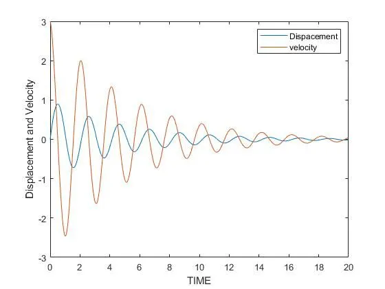
Output after solving the ODE.
1.The Plot of Displacement v/s Time; Velocity v/s Time.
Animation:
Here is the link to the animation of the oscillation of pendulum for the solved ODE: