Week 3 - Solving second order ODEs

Aim: 1) Write a MATLAB code to plot the angular displacement and time using ordinary differential equations.

2) Create an animation of simple pendulum.

Theory:

In mathematics, an ordinary differential equation(ODE) is a differential equation containing one or more functions of one independent variable and the derivatives of those functions. The term ordinary is used in contrast with the term partial differential equation which may be with respect to more than one independent variable.

An ordinary differential equation for simple pendulum is given by,

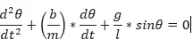
Where b = damping

m = mass

g = gravity

l = length

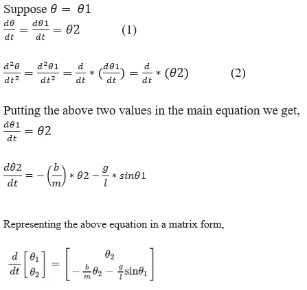
Representing the above equation in a matrix form,

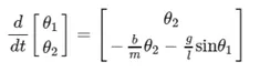
By using the above equation and ode45 solver we can solve the differential equation in a matlab.

Matlab Code:

clear all

close all

clc

b = 0.05;

g = 9.81;

l = 1;

m = 1;

% initial condition

theta_0 = [0;3];

% time points

t_span = linspace(0,20,500);

% solve ODE

[t,results] = ode45(@(t,theta) ode_func(t,theta,b,g,l,m),t_span,theta_0);

plot(t,results(:,1))

hold on

plot(t,results(:,2))

title('Motion of pendulum')

xlabel('time')

ylabel('Plot')

legend('Displacement','Angular Velocity')

Displacement = results(:,1);

% count command for iterations.

ct = 1;

for i = 1:length(Displacement)

omega = Displacement(i);

% Fixed co-ordinates of one end of simple pendulum

x0 = 0;

y0 =0;

% moving co-ordinates of bob

x1 = l*cos((3*pi/2)+omega);

y1 = l*sin((3*pi/2)+omega);

%Plotting of the bob motion

figure(2)

plot([x0 x1],[y0 y1],'linewidth',3,'color','g');

hold on;

plot(x1,y1,'o','markers',15,'MarkerFaceColor','r');

hold on;

plot([-3,3],[0 0],'linewidth',2,'color','b');

hold off

axis([-3 3 -2 2])

grid on

title('Animation of pendulum')

pause(0.01)

M(ct) = getframe(gcf);

ct = ct+1;

end

% To create an animation of simple pendulum

movie(M)

videofile = VideoWriter('Simple_pendulum.avi','Uncompressed AVI');

open(videofile)

writeVideo(videofile,M)

close(videofile)

ODE45 function code:

function [dtheta_dt] = ode_func(t,theta,b,g,l,m)

theta1 = theta(1)

theta2 = theta(2)

dtheta1_dt = theta2;

dtheta2_dt = -(b/m)*theta2 - (g/l)*sin(theta1);

dtheta_dt = [dtheta1_dt; dtheta2_dt]

end

Explanation of the code:

• The clear all, close all, clc are the commands to clear the workspace and command window as you run the code again and again.
• The values of the input arguments like gravity, length of the pendulum, mass of the ball, damping coefficient are defined.
• Initial conditions are defined in a variable theta_0 = [0;3]. Here 0 represents the initial displacement while 3 represents the initial velocity.
• t_span variable is used to create an array of timepoints using linspace command. The time will vary between 0 to 20 sec for 500 values.
• The differential equation in a matrix form is represented in matlab using ode45 function.
• MATLAB’s standard solver for ordinary differential equations (ODEs) is the function ode45. This function implements a Runge-Kutta method with a variable time step for efficient computation. ode45 is designed to handle the following general problem:

dx dt = f(t, x), x(t0) = x0, (1) where t is the independent variable, x is a vector of dependent variables to be found and f(t, x) is a function of t and x. The mathematical problem is specified when the vector of functions on the right-hand side of Eq. (1), f(t, x), is set and the initial conditions, x = x0 at time t0 are given

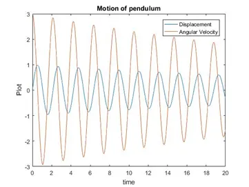
• Finally the plot of results(Angular displacement and angular velocity) are plotted.
• Figure 1 is going to tell how the damping is done for the pendulum. The angular velocity and angular displacement will stop at the end of the function.
• To animate the motion of simple pendulum, a for loop is used to create the specified set of points to keep the bob at different positions.
• X0 and y0 be the fixed end of the string while x1,y1 be the different position of the bob.
• At each and every position of the bob, ct command is used to count each and every position of the bob and store the data.
• At the end of the for loop, there will be set of points for position of the bob.
• Movie(M) is used to create a film of the stored data of the motion of pendulum.
• Video writer command specifies the name of the file and type of data stored in it.
• Writevideo command is used to create the video animation by using M file.
• Close command is used to close the video file.

Results:

Youtube link for animation of simple pendulum.

https://youtu.be/nxViecZCu9E

Conclusion: The angular velocity and displacement are calculated for simple pendulum. The second order differential equation is solved to simple differential equation using ode45 function. The animation of simple pendulum is created for different positions of the bob.