SOLVING SECOND ORDER ODEs

AIM : To write a python program for the simulation of movement of simple pendulum.

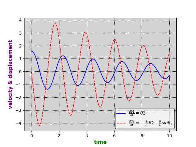
OBJECTIVE : 1.To generate the combined graph between velocity,displacement and time.

2.To simulate the movement of simple pendulum which moves according to second order differential equation.

THEORY :

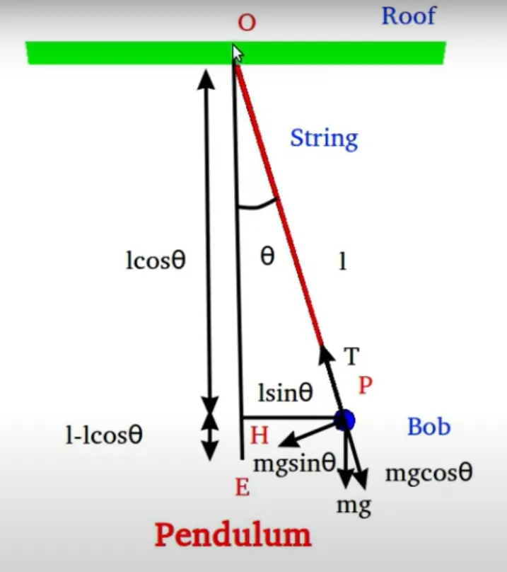
A simple pendulum consists of a mass m hanging from a string of length L and fixed at a pivot point P. When displaced to an initial angle and released, the pendulum will swing back and forth with periodic motion.

Second order differential equation:

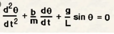
where,

b = damping coefficient

m = mass of the ball(kg)

g = gravity(m/s^2)

L = length of the string(m)

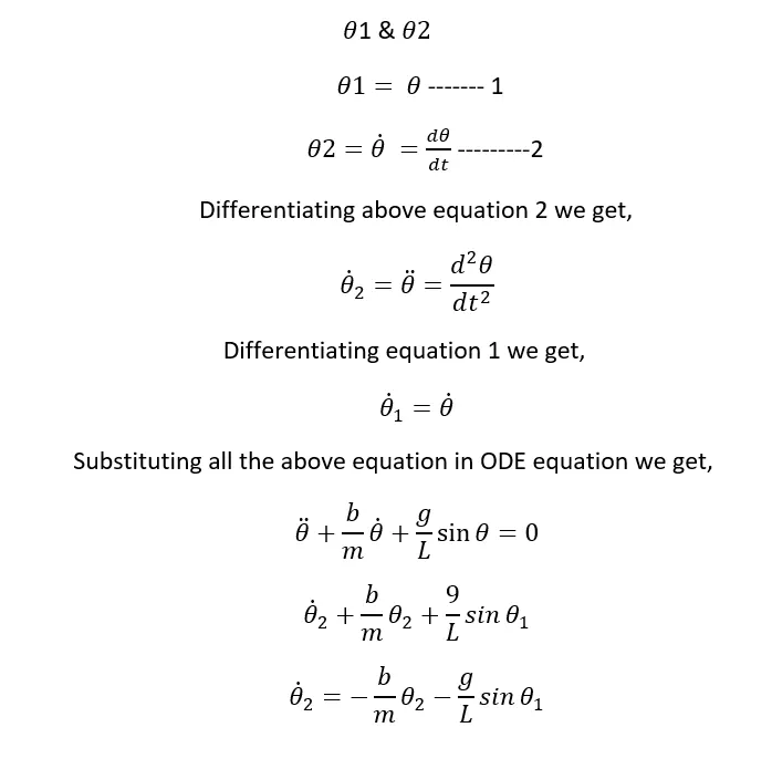
The above equation is differential equation of second order and in order to split it into two first order differential equation we need two variables.

PROCEDURE :

1.Import the matplotlib,numpy and math libraries for plotting and calculating math operations.

2.Import "odeint" from scipy.integrate module to solve the differential equation.

3.Define the function and write the logic to split the second order differential equation into two first order differential equations.

4.Call the function and define the variables.

5.Plot the graph between velocity and time.

PYTHON PROGRAM CODE:

import matplotlib.pyplot as plt
import numpy as np
import math
from scipy.integrate import odeint


#input

b = 0.05   #damping(kg/m^2-s)
g = 9.81   #gravity(m/s^2)
l = 1      #length (m)
m = 1    #mass (kg)
theta1 = math.pi/2 #initial angle
theta2 = 0         #initial angular velocity
theta_init = (theta1,theta2)
t = np.linspace(0,10,500)  #timesteps


def pendulum(theta_init,t,l = 1,m = 0.1,b = 0.02,g = 9.81):
	theta_dot_1 = theta_init[1]
	theta_dot_2 = -b/m * theta_init[1] - g/l *math.sin(theta_init[0])
	dtheta_dt = [theta_dot_1,theta_dot_2]
	return dtheta_dt



#to solve ode
theta = odeint(pendulum,theta_init,t,args = (l,m,b,g))
 
ax=plt.axes()
ax.set_facecolor('lightgrey')
plt.plot(t,theta[:,0],'b-',label=r'$frac{dtheta1}{dt}=theta2$')
plt.plot(t,theta[:,1],'r--',label=r'$frac{dtheta2}{dt}=-frac{b}{m}theta2-frac{g}{L}sintheta_1$')
plt.xlabel('time',color='green',fontsize='large',fontweight='bold')
plt.ylabel('velocity & displacement',color='purple',fontsize='large',fontweight='bold')
plt.legend(loc='best',edgecolor='black',framealpha=0.7)
plt.grid(True,color='black',linestyle='dotted')

plt.show()


#Simulation of simple pendulum
c=1
for THETA in theta[:,0]:
	x0 = 0
	y0 = 0
	x1 = l*math.sin(THETA)
	y1 = -l*math.cos(THETA)
	print(THETA)
	filename='test%05d.png' %c
	c = c+1

	plt.figure()
	plt.plot([-1,1],[1,1],'red',linewidth = 4)
	plt.plot([x0,x1],[1,y1],'black')
	plt.plot(0,1,'o',markersize=5)
	plt.plot(x1,y1,'o',markersize=30,color='orange')
	plt.xlim([-1.5,1.5])
	plt.ylim([-1.5,1.5])
	plt.savefig(filename)

OUTPUT :

Different theta values:

1.5707963267948966 1.5688271540472822 1.5629221513339004 1.5530854543642596 1.5393215253124788 1.5216356842095402 1.5000347349728418 1.4745277734744622 1.4451271920080335 1.4118498191456192 1.374718244805943 1.333762280460509 1.2890205465285114 1.2405421761958786 1.1883885672400933 1.1326351836881274 1.0733733343558398 1.010711877669264 0.9447787853755967 0.8757225138709295 0.8037130615903232 0.7289426965807121 0.6516262439108131 0.5720008931866193 0.49032545581713827 0.40687906101150595 0.3219592745814811 0.235879670624841 0.14896689317523856 0.061557288549582936 -0.026006788533812282 -0.11338087244438644 -0.20022236711718072 -0.28619445861347786 -0.370969829073008 -0.45423405602121636 -0.5356885897112449 -0.615053228569574 -0.6920680483391384 -0.766494761188853 -0.8381175007651418 -0.9067430704677604 -0.9722007027473304 -1.0343413825802659 -1.0930368095885825 -1.1481780765469907 -1.1996741355319456 -1.2474501207192044 -1.291445597504443 -1.3316127932712056 -1.3679148569470096 -1.4003241922015068 -1.428820894769404 -1.4533913175808322 -1.4740267873722586 -1.4907224836994761 -1.5034764827299572 -1.5122889843514462 -1.517161717569384 -1.51809753726982 -1.5151001849305408 -1.508174250491178 -1.4973253084040943 -1.4825602333822163 -1.463887699928237 -1.441318855217833 -1.4148681656556104 -1.3845544298541281 -1.3504019493421744 -1.3124418438667231 -1.2707134968983123 -1.2252661024353244 -1.1761602930016002 -1.1234698081325036 -1.0672831534134661 -1.0077052142247105 -0.9448587527717327 -0.8788857244336123 -0.8099483591471386 -0.7382299210587446

GRAPH:

VELOCITY & DISPLACEMENT V/S TIME

ANIMATED VIDEO:

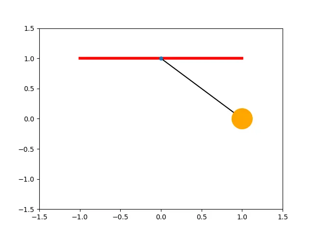
VIDEO LINK:

https://www.veed.io/download/89e868c4-9638-44a8-8c9f-c57d6aa8185b

RESULT :

Simulating the movement of simple pendulum has been done using python code.