Solving second order ODEs using Python

Objective: To solve ODE of simple pendulum using python.

Problem Statement: It is necessary to solve ODE for a respective problem. It is manual process to solve ODE and time consuming to plot. It will be very easy if it can be written into computer understandable code.

Theory: A function was defined for calculating the angular displacement and velocity of simple pendulum at different time intervals. The second-order differential equation defining the motion of pendulum

`(d^2 θ)/(dt^2 )+b/m.dθ/dt+g/l.sin⁡θ=0`

b = damping.

m = mass.

g = gravity.

l = length.

Above ODE is split into 2 single order differential equations ( `(dθ_1)/dt=θ_2`) and (`(dθ_2)/dt=-b/m.θ_2-g/l.sin⁡θ_1`) and defined within the function.

Procedure:

• Importing math,matplotlib,numpy,image,glob libraries
• Defining 1^st order ODE’s .
• Passing initial values.
  1. b = 0.05
  2. g = 9.81
  3. l = 1
  4. m = 0.5
• Passing initial condition for theta1 & theta2.
• Passing (t) for 15 sec and dividing it into 300 times.
• Solving ODE using odeint by calling defined ODE’s.
• Plotting Angular displacement and Velocity Vs Time.
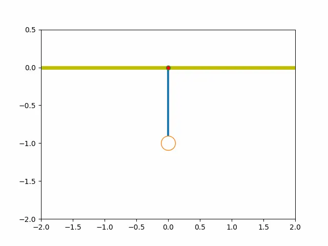
• Plotting state of simple pendulum on Graph and saving images.
• Sewing all images together to create GIF of simple pendulum motion.

Program:

import numpy as np
from scipy.integrate import odeint
import matplotlib.pyplot as plt
import math
from PIL import Image
import glob
#function that returns dz/dt
def model(theta,t,b,g,l,m):
	theta1 = theta[0]
	theta2 = theta[1]
	dtheta1_dt = theta2
	dtheta2_dt = -(b/m)*theta2 - (g/l)*math.sin(theta1)
	dtheta_dt = [dtheta1_dt,dtheta2_dt]
	return dtheta_dt
b = 0.05
g = 9.81
l = 1
m = 0.5
#initial condition
theta_0 = [0,3]
#time points
t = np.linspace(0,15,300)
#solve ODE
theta = odeint(model,theta_0,t,args = (b,g,l,m))
#print(theta)
#plot results
plt.plot(t,theta[:,0],'b-', label = r'$frac {dtheta_1}{dt}=theta2$')
plt.plot(t,theta[:,1],'r--',label = r'$frac{dtheta2}{dt}= -frac{b}{m}theta_2-frac{g}{l}sintheta_1$')
plt.ylabel('plot')
plt.xlabel('time')
plt.legend(loc = 'best')
#plt.savefig('Graph_disvelo')
plt.show()
#plotting simple pendulum on graph at each angle.
x = theta[0,1]
y=theta[:,0]
ct=1
for ang in y :
	x1=0;y1=0
	x2=l*math.sin(ang)
	y2=-l*math.cos(ang) 
	plt.figure()
	plt.plot([-2.0,2.0],[0,0],'y',linewidth=5)
	plt.plot([x1,x2],[y1,y2],linewidth=3)
	plt.plot(x2,y2,'o',markersize=20,markerfacecolor='w')
	plt.plot(x1,y1,'o',markersize=6,markerfacecolor='r')
	plt.xlim([-2.0,2.0])
	plt.ylim([-2.0,0.5])
	filename = 'test%05d.png'%ct
	plt.savefig(filename)
	ct=ct+1
	#creating 'gif' from the images saved
	frames = []
	imgs = glob.glob("*.png")
	for i in imgs:
		new_frame = Image.open(i)
		frames.append(new_frame)
	# Save into a GIF file that loops forever
	frames[0].save('png_to_gif.gif', format='GIF',
		append_images=frames[1:],
		save_all=True,
		duration=60, loop=0)

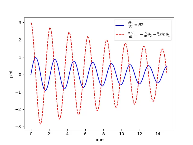
Results: The graph below shows the variation of Angular displacement and velocity of pendulum w.r.t time.

Blue line—Displacement curve.

Redline—Velocity curve.

Below is the animation of simple pendulum using image and glob libraries.

Conclusion:Hence ODE of simple pendulum is solved using python and respective plots were plotted with respect to time.