Week 3 - Solving second order ODEs

Project Made By – Piyush Mishra

Aim

The main purpose of this project is to perform integration on Ordinary Differential Equations (ODEs) of simple pendulum via Python Coding

Governing Equations

General Equation for Simple Pendulum

(d²θ/dt²) + (c/m) (dθ/dt) + (g/l) Sin (θ) = 0

Where -->

c = Damping coefficient

g = Gravity

l = Length of Pendulum

m = Mass of bob

(dθ/dt) = Displacement of Pendulum

(d²θ/dt²) = Velocity of pendulum

Θ = angle made by mean position of pendulum

Physics Involve

Ideal Simple Pendulum à A simple pendulum is defined to have a point mass, also known as the pendulum bob, which is suspended from a string of length L with negligible mass. Here, the only forces acting on the bob are the force of gravity (i.e., the weight of the bob) and tension from the string.

Damping In Pendulum à When the motion of an oscillator reduces due to an external force, the oscillator and its motion are damped. These periodic motions of gradually decreasing amplitude are damped simple harmonic motion.

Simple Harmonic Motion (SHM) à In mechanics and physics, simple harmonic motion is a special type of periodic motion where the restoring force on the moving object is directly proportional to the object's displacement magnitude and acts towards the object's equilibrium position

Objectives of the Project

The Objectives for the Project are to be done by Python Programming. They are:

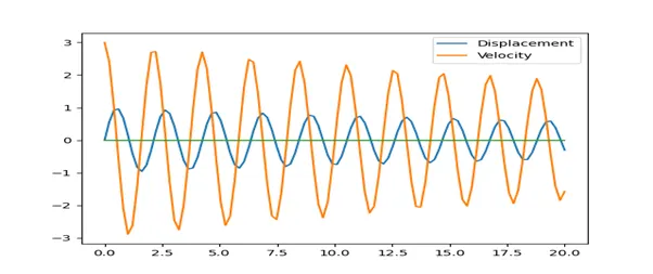
1. Is to plot graph showing the variation of Displacement and Velocity of a simple pendulum with respect to time.
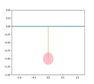
2. Is to animate the Simple Pendulum

Body of Content

Python Programing is used here with explanation:

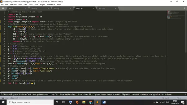
# Importing Required Libaraies
import math
import matplotlib.pyplot as pt
import numpy as ny
from scipy.integrate import odeint # For integrating the ODEs 

# Defining system/function that need to be Integrated
def sys(theta,t,c,g,m,l): # Defining Fuction for which integration is done
	t1 = theta[0] # Defining each value of array so that individual operations can take place
	t2 = theta[1]
	dt1 = t2 # Defining values for operation for Velocity 
	dt2 = -(c/m)*t2 - (g/l)*math.sin(t1) # Defining values for operation for Displacement
	dt = [dt1,dt2] # Defining array while putting things in array 
	return dt # Returning values for dt array

# Given Input
c = 0.05 # Damping coefficient
g = 9.81 # Gravity (in m/s2)
l = 1 # Length of Pendulum (in m)
m = 1 # Mass of bob (in kg)	
ct = 1 # A counter variable to save the file name, it is being defined as global variable as ct would be counter after every time function is being called
t0 = [0,math.pi*0.95492965856] # Initial Condition for Displacement (0 m) & Velocity (3 rad = 0.95492965856 X pie)
t = ny.linspace(0,20,100) # Defining array for values that need to be integrate
theta = odeint(sys,t0,t,args = (c,g,m,l)) # Odeint function which is used to Integrate 

# Ploting grap
pt.plot(t,theta[:,0], label="Displacement") # (theta[:,0]) are the first position for the array
pt.plot(t,theta[:,1], label="Velocity")
pt.plot([0,20],[0,0])
pt.legend()
pt.show()

# Animation for Pendulum <As it is already done perviously so it is hidden for less consumption for screenshot>
for T in theta[:,0]:
	x0 = 0 # Fix position of tip of pendulum 
	y0 = 0
	x1 = l*math.sin(T) # Position of root which keeps changing according value of displacemnet 
	y1 = -l*math.cos(T)
	filename = 'pen' + str(ct) + '.png' # Defining a string variable for saving name for graph
	ct = ct + 1 # Appending value for ct so that overwriting is avoided
	# Ploting grap
	pt.figure()
	pt.plot([-1.25,1.25],[0,0], linewidth=2)
	pt.plot(x1,y1, 'o', markersize = 50, color ='pink')
	pt.plot([x0,x1],[y0,y1])
	pt.xlim([-1.25,1.25])
	pt.ylim([-1.5,0.5])
	pt.savefig(filename)

It’s Output

Graph

Animation

(Animation is made by other Software, not by Coding). Although here it is quite difficult to attach the animated gif

Conclusion

There is not much to conclude but we have not only integrated the Ordinary Differential Equations (ODEs) of the simple pendulum but also, plotted the graph showing the variation of Displacement and Velocity of a simple pendulum with respect to time.

Lastly, we were also able to animate the Simple Pendulum