Week 3 - Solving second order ODEs

Problem Statement:

Write a program in Python to solve a second-order 'Ordinary differential equation' that represents the equation of motion of a simple pendulum with damping and create an animation of this motion.

Theory :

The figure shows an idealized pendulum, with a "massless" string or rod of length 'L' and a bob of mass 'm'. When the bob is moved from its rest position and let go, it swings back and forth. The time it takes the pendulum to swing from its farthest right position to its farthest left position and back to its next farthest right position is the period of the pendulum. The primary forces acting on the bob are the gravitational force that makes it move in the first place and the force exerted by the string to keep it moving along a circular path. In addition, there may be a damping force from friction at the pivot or air resistance, or both.

Mathematically the equation of motion of a simple pendulum with damping can be derived as -

Let theta(t) be the corresponding angle with respect to the vertical. The figure shows tangential and radial components of gravitational force on the pendulum bob. The radial component is exactly balanced by the force exerted by the string, so the only relevant force producing the motion is the tangential component of the gravitational force. For the moment, we ignore the damping force, if any.

The gravitational force is directed downward and has magnitude mg (mass x acceleration), where g is the gravitational acceleration constant 9.807 meters/sec2 near sea level. Thus, the force acting in the tangential direction is -mg sin(theta). (The negative sign is because this force is in the negative direction when theta is positive and vice versa.) Since this force is mass x acceleration, it follows that

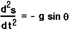
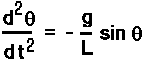
Now s and theta are related as arc length and central angle in a circle of radius L: s = L theta. Thus, the second derivative of s is L times the second derivative of theta. That brings us to our undamped model differential equation with a single dependent variable, the angular displacement theta:

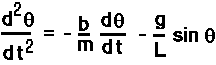
Next, we add damping to the model. We make the simplest possible assumption about the damping force, that it is proportional to velocity. Since arc length and central angle are themselves proportional (with proportionality constant L), it makes no difference whether we use linear or angular velocity. Having selected theta as our dependent variable, we will represent the damping is proportional to angular velocity, say, -b (d theta / dt). The negative sign is because the damping force has to be opposite the direction of motion. When we include this term in the model, our equation becomes

When we bring all the terms to the left-hand side, our model equation becomes -

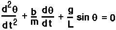
The equation is a second order ODE. To solve it we convert it into two first order ODEs -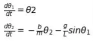

Using the odeint function of the scipy module, we solve these equations for theta with respect to time.

Program -

import math
import matplotlib.pyplot as plt 
import numpy as np 
from scipy.integrate import odeint

#user defined function to define the two first order ODEs
def model(theta,t,b,g,l,m):
	theta1 = theta[0]
	theta2 = theta[1]
	dtheta1_dt = theta2
	dtheta2_dt = -(b/m)*theta2 - (g/l)*math.sin(theta1)
	dtheta_dt = [dtheta1_dt, dtheta2_dt]
	return dtheta_dt
#inputs 
b = 0.05 #damping
g = 9.81 #gravitational acceleration
l = 1 #length of massless string
m = 1 #mass of bob

#initial conditions (angular disp, angular vel)
theta_0 = [0, 3]

#time array using numpy module
t = np.linspace(0,20,150)

#find values of theta using scipy function odeint. giving inputs 
#of our system/equations/model, initial cond, time and basic inputs
theta = odeint(model, theta_0, t, args = (b,g,l,m))

ct = 1 #counter initialization

#to find x&y coordinates of the bob at each value of theta w.r.t time
for i in range(0, 150):
	x_coord = l*math.cos(3*math.pi/2 + theta[i,0])
	y_coord = l*math.sin(3*math.pi/2 + theta[i,0])


	filename = 'frame%05d.png' %ct # to set filename. %05d means 5 digits after frame i.e. frame00000.png
	ct = ct + 1 # counter increment by 1

	#plotting 
	plt.figure()
	plt.plot([-2,2],[0,0],'r-') #base line
	plt.plot(x_coord,y_coord,'ro', markersize = 6.0) #bob
	plt.plot([0,x_coord],[0,y_coord],'b-') #string
	plt.xlim([-2,2]) # limtis to be set to axes
	plt.ylim([-2,2])	
	plt.savefig(filename) #saving each figure window after plotting

-> We create a user defined function to model our system of equations that consist of the two first order ODEs derived from our main equation.

-> Define inputs such as damping, length of string, mass of bob and gravity. Also initial conditions of angular displacement and angular velocity at time = 0s are defined.

-> Using the numpy module we create a time array from 0-20s with 150 values between the time interval.

-> Next, we find the values of theta w.r.t time using the odeint function from the scipy module by giving the inputs, initial conditions, system of equations and time array. On a 2D plot, the values of angular velocity and displacement w.r.t time are -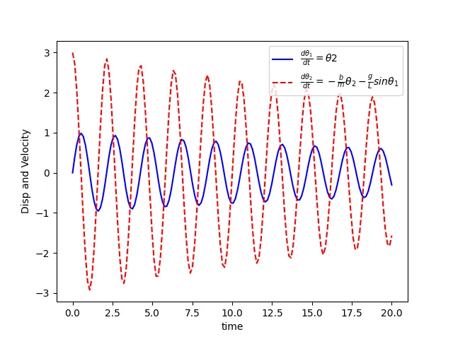

-> using a for loop we find the coordinates of the bob for each value of theta w.r.t time. These values are then plotted with base coordinates (0,0) to represent the string. The coordinates are further plotted as a marker to represent the bob. And a base line is plotted from -2 to 2 on x-axis.

-> Each figure is saved and given a filename 'frame(followed by five digits)'. The digits are initialised at 1 using a counter variable before the start of the for loop and incremented by 1 inside the for loop.

-> These figures are then stitched together using ImageMagick from command prompt to output an animation in the format of our choice -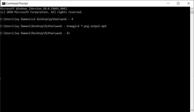

Youtube link -

https://youtu.be/QGbyzyYVE5k