Week 3 - Solving second order ODEs

Week 3 - Solving Second Order Differential Equations (ODEs)

Objective:

To write a python program that solves the second order differential equation (ODE) that describes the position of a pendulum with respect to time.

Problem Statement:

To solve a second ODE, we need to rewrite the equation as two first order differential equations. The second ODE to be solved is given below:

`(d^2theta)/dt^2 + b/m (d(theta))/dt + g/lsintheta = 0`

where,

`theta`- Angular Displacement (radians)

`b`- Damping Coefficient (`(Ns)/m`)

`m` - Mass of Pendulum (kg)

`g` - Acceleration due to gravity (`m/s^2`)

`l` - Length of pendulum string (m)

If this differential equation is solved, we will be able to determine the displacement and hence velocity of the pendulum at any given time. Using this information, we can write a simple program that captures snapshots of the displacement of the pendulum to create an animation of the pendulum motion.

Solution:

To solve the second ODE, we need to rewrite the equation as two first ODEs instead.

Let `theta = theta_1`

`(d(theta))/dt = (d(theta_1))/dt = theta_2` - Equation 1

`(d^2theta)/dt^2 = (d^2(theta_1))/dt^2 = (d(theta_2))/dt` - Equation 2

`(d^2theta_1)/dt^2 + b/m (d(theta_1))/dt + g/lsintheta_1 = 0`

`(d(theta_2))/dt^2 + b/m (d(theta_2))/dt + g/lsintheta_1 = 0`

The two first ODEs are given below:

`(d(theta_1))/dt = theta_2`

`(d(theta_2))/dt = (d^2(theta_1))/dt^2 = -b/m(d(theta_1))/dt - g/lsintheta_1`

Procedure:

First, open all the necessary python libraries in to a new script file. Four main libraries are required for this assignment. One of the main libraries is the "scipy.integrate" library from which we need to import the "odeint" function. This function enables the solving of ODEs. These libraries are shown in the section of code given below:

import numpy as np 
import matplotlib.pyplot as plt 
import math
from scipy.integrate import odeint

Next, create a function that will solve for the instantaneous velocity of the pendulum using certain arguments. The arguments are listed below:

• angular displacement
• time
• damping coefficient
• gravity
• length
• mass

These arguments are required as they are the parameters in the ODE for the motion of the pendulum. Then, the two first order differential equations are entered in to the function using the arguments. Variables "theta1" and "theta2" are created which correspond to the same angular unknowns used to rewrite the second ODE as two first ODEs. In this case, "theta1" is the angular displacement, and "theta2" is the rate of change of "theta1" which is equivalent to the velocity. The function will calculate the angular velocity. This is shown in the section of code below:

# Function to return the velocity
def velocity(theta, t, b, g, l, m):
	theta1 = theta[0]
	theta2 = theta[1]
	dtheta1_dt = theta2
	dtheta2_dt = -(b/m)*theta2 - (g/l)*math.sin(theta1)

	dtheta_dt = [dtheta1_dt, dtheta2_dt]
	return dtheta_dt

Then, the parameters of the pendulum are defined. These parameters are the aforementioned values for the damping coefficient, gravity, length, and mass of the pendulum. The same values as required by this assignment are used. This is shown in the section of code given below:

# Parameters of pendulum
b = 0.05
g = 9.81
l = 1
m = 1

Next, the initial conditions of the pendulum are defined. Two conditions need to be defined. The first is the initial displacement, and the second is the initial velocity. As required by the assignment, an initial displacement and initial velocity of 0 radians and 3 metres per second are used. These values are entered in an array for the variable "theta_0".

Then, a time array is created between 0 and 20 seconds using the "linspace" command found in the "numpy" library. This command creates equally spaced values between 0 and 20. In my case, my time array will have 160 equally spaced values.

Afterwards, the ODE is solved using the "odeint" command. This command requires certain inputs to be inserted in a given order as per its syntax. The "odeint" command requires a function, the initial conditions, a time array, and the argument parameters. This is shown in the section of code given below:

# Initial Conditions - Displacement & Velocity
theta_0 = [0, 3]

# Time Points
t = np.linspace(0, 20, 160)

# Solve ODE
theta = odeint(velocity, theta_0, t, args = (b, g, l, m))

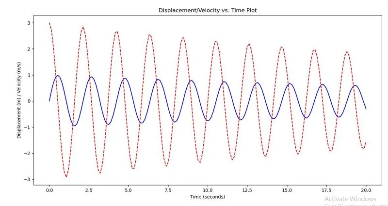
Now that we have solved the second ODE, we have a set of displacement and velocity arrays for a 20 second period. These results can be plotted in a graph. In this case, two plots will be plotted. The first plot will show the displacement against the time, and the second plot will show the velocity against the time. In order to plot these graphs, we need to retrieve the data from the "theta" array. The first column of this array contains the displacement data, and the second column contains the velocity data. In order to retrieve this data, indexing is used e.g. "theta[:,0]".

To differentiate the plots, different markers are used with different colors. The first plot (displacement) will have a blue color line with single dots whereas the second plot (velocity) will have a red color line with double dots. For better presentation, plot titles, and axis titles are also added. The plot is printed. This is shown in the section of code given below:

# Plot Results
plt.plot(t, theta[:,0], 'b-')
plt.plot(t, theta[:,1], 'r--')
plt.title('Displacement/Velocity vs. Time Plot')
plt.xlabel('Time (seconds)')
plt.ylabel('Displacement (m) / Velocity (m/s)')
plt.show()

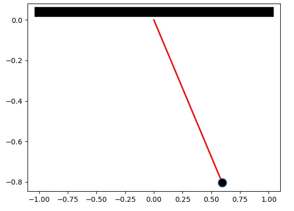
Finally, the animation of the pendulum can now be created with the displacement and velocity data in the "theta" array. First, a new variable for displacement is created called "disp" which retrieves the displacement values from the "theta" array. The "ct" variable is created and set to 1. This value acts as a counter for the frames of the animation.

A for loop is started where for every value in the "disp" variable, the positions of the pendulum are calculated. Variables for the x and y coordinates are created for two situations. The first situation is the starting position where the pendulum is at equilibrium i.e. at zero displacement. This position is considered the origin point. The second situation is when the pendulum is in motion. In this case, the x and y coordinate of the pendulum bob is determined using Pythagoras' theorem. In this calculation, we needed to subtract "pi" or 180 degrees from the calculation.

Then a variable called "filename" is created which converts the counter value to a string and adds ".png" to the end. This variable just creates the files for the animation of the pendulum. Each file represents a frame in the animation. The counter value is then commanded to increase by 1 for each iteration of the for loop. The plot is then commanded to appear in a new figure.

To show the animation of the pendulum, a fixed support, pendulum string, and pendulum bob are created in the plots using markers and line widths and line colors. The positions of each of these items are given coordinates to appear in specific points in the plot to appear like an actual pendulum. Finally, the plots are saved according to the "filename" variable at each iteration of the for loop.

disp = theta[:,0]

print(disp)

# Animation of Pendulum

ct = 1
for i in disp:
	# Starting Pendulum Position
	x0 = 0
	y0 = 0

	# Position of Pendulum as it moves
	x1 = l*(math.sin(i-math.pi))
	y1 = l*(math.cos(i-math.pi))

	filename = str(ct) + ".png"
	ct = ct + 1

	plt.figure()

	# Fixed Support
	plt.plot([-1, 1], [0.04, 0.04], color='black', linewidth=14)

	# Pendulum string position from fixed support
	plt.plot([x0, x1], [y0, y1], color='red', linewidth=2)

	# Pendulum Bob
	plt.plot(x1, y1, marker='o', markerfacecolor='black', markersize=12)
	
	plt.savefig(filename)

Once all the plots are created, they are moved to a dedicated folder. Using the Cygwin terminal and "ImageMagick Display" software, the command "magick * output.gif" is used to create an animation from all the plots.

Results:

The plot is shown in the image given below:

The animation of the pendulum is shown in the image below:

Errors Faced:

During the ploting of the animation file, the positions of the pendulum were incorrectly calculated. The angular values in the "disp" array were not subtracted by 180 degrees. This resulted in the animation file looking strange. The animation was only moving to one side and was not oscillating as it should.

In addition, in the time array, initially only 20 equally spaced values were used. This was not wrong, but resulted in an animation that was not smooth.

Conclusion:

In conclusion, the second ODE of the pendulum was solved. The solved ODE was used to plot the displacement and velocity characteristics of a pendulum against the time. The calculated values for the displacement were used to successfully create an animation plot which showed how the pendulum moves for the specified time array.

The python script, plot of the results and the pendulum animation are attached to this assignment.