Week 3 - Solving second order ODEs

In Engineering, ODE is used to describe the transient behavior of a system. A simple example is a pendulum

The way the pendulum moves depends on the Newtons second law. When this law is written down, we get a second order Ordinary Differential Equation that describes the position of the "ball" w.r.t time.

Similarly, there are hundreds of ODEs that describe key phenomena and if you have the ability to solve these equations then you will be able to simulate any of these systems.

Your objective is to write a program that solves the following ODE. This ODE represents the equation of motion of a simple pendulum with damping.

Second order differential equation is a specific type of differential equation that consists of a derivative of a function of order 2 and no other higher-order derivative of the function appears in the equation.

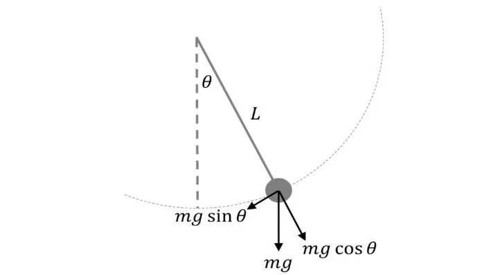
A simple pendulum consists of a ball (point-mass) m hanging from a (massless) string of length L and fixed at a pivot point P. When displaced to an initial angle and released, the pendulum will swing back and forth with periodic motion. By applying Newton's second law for rotational systems, the equation of motion for the pendulum may be obtained.

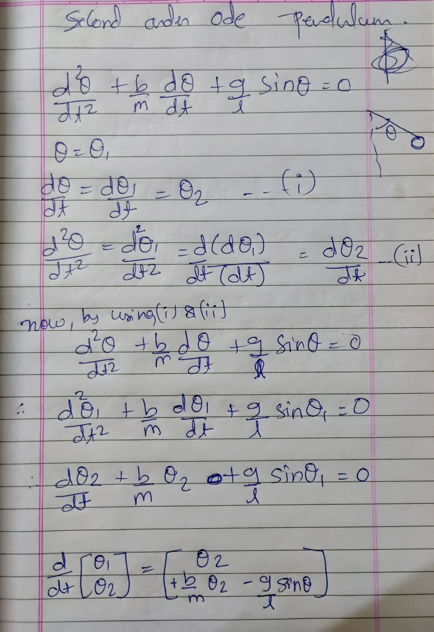
Second order Differential Equation can be simplified in :

where as ,

𝜽 is the angular displacement

𝒃 is the damping coefficient

𝒎 is the mass of the ball

𝒈 is the acceleration due to gravity

𝒍 is the length of the pendulum

now this equations will be applied in Python Programming using sublime text editor, lets program it step by steps :

import math

import matplotlib.pyplot as plt

import numpy as np

from scipy.integrate import odeint

#functions returns dz/dt

def model(theta, t, b, g, l, m):

theta1 = theta[0]

theta2 = theta[1]

dtheta1_dt = theta2

dtheta2_dt = -(b/m)*theta2 - (g/l)*math.sin(theta1)

dtheta_dt = [dtheta1_dt, dtheta2_dt]

return dtheta_dt

#initial condition

b = 0.05 # damping co-efficient

g = 9.81 #gravitational

l = 1 #(mtr)

m = 1 #(kg)

theta_0 = [0,3]

#time points

t = np.linspace(0,20,200)

#solve ode

theta = odeint(model, theta_0, t, args = (b, g, l, m))

ang_disp = theta[:, 0]

ang_vel = theta[:, 1]

#plotting results

plt.plot(t, ang_disp, 'b-', label='angular displacement')

plt.plot(t, ang_vel, 'r-', label='angular velocity')

plt.legend()

plt.xlabel('time')

plt.ylabel('displacement and velocity')

plt.title('Second ODE of Simple Pendulum')

plt.show()

# To create Animation

ct = 1

x0 = 0

y0 = 0

for i in theta[:,0]:

x1=x0+(1*math.sin(i))

y1=y0+(-1*math.cos(i))

filename = str(ct)+'.png'

ct = ct+1

plt.figure()

plt.plot([-1,1],[0,0],"yellow")

plt.plot([x0,x1],[y0,y1],"red")

plt.plot(x1,y1,'o',markersize = '10')

plt.xlim([-1.5,1.5])

plt.ylim([-1.5,1.5])

plt.savefig(filename)

plt.plot()

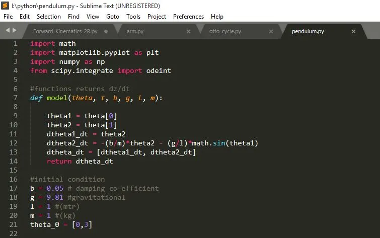
step 1 : Importing all the required libraries such as math, matplotlib, numpy and scipy for ode solution.

step 2 : Defining the ode model with theta, time, damping, gravity, length and mass and also the differential equation is calculated and simplified.

step 3 : Initial conditions are given for b,g,l,m and initial theta angle for angular velocity and displacement.

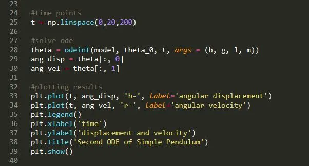
step 4 : using linspace function a time interval is created for 200 points between 0 and 20.

solving the ode using odeint function from scipy eventually between the time intervals of angular displacement and angular velocity.

step 5 : Plotting and generating the results for both displacement and velocity.

Plot results :

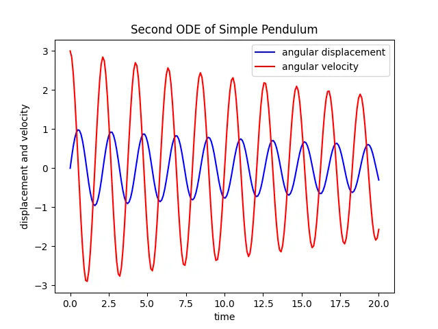
If we take a look on the plots its visible that the angular displacement is starting from 0 and it fluctuates from 1 to -1 displacement and as its is moving with time its motion gets minimizing similarly with angular velocity it is starting from 3 to -3 and as the time passes its motion gets reduced to near about 2 to -2 displacement.

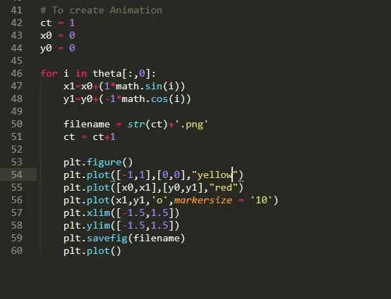
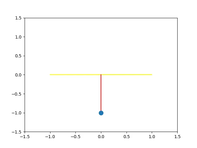
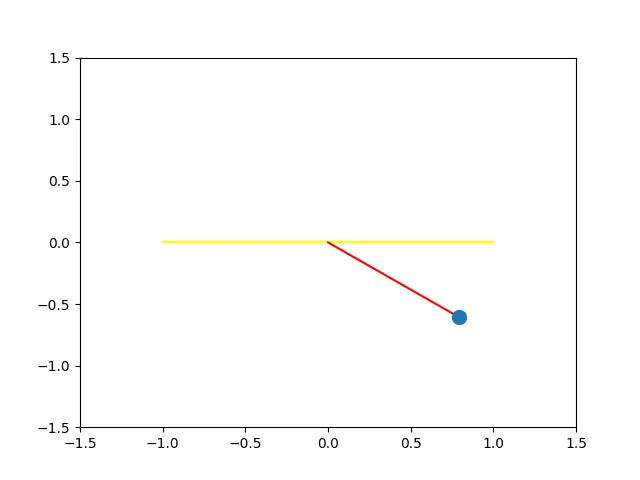
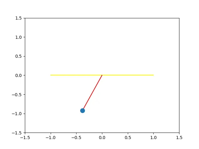
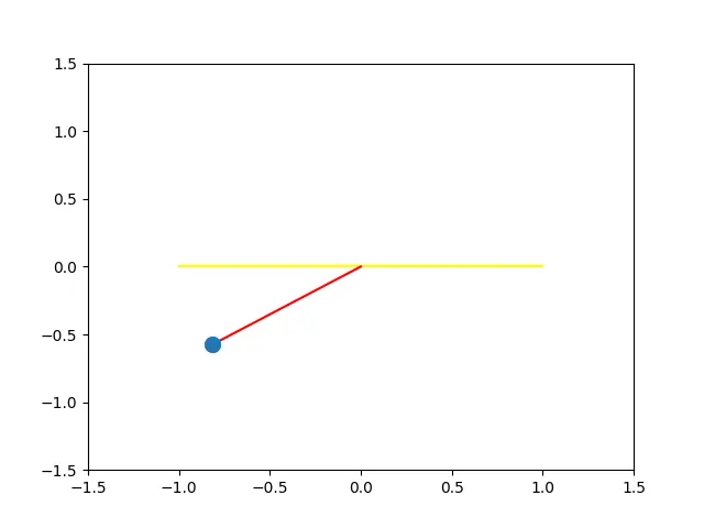
step 6 : Animation Generation using the plots position with time . The code deals with the creation of pendulum animation. The initial position of the pendulum rod is defined; then a counter is also defined which will let us create and store each image to each position of the pendulum. The position of rod and length is located using yellow and red color for both rod and base. Axes limit is been defined for both x and y as -1.5 to 1.5. In the last the Figure is saved for each time given.

Total 200 images are generated and from those images here few are attached and for the rest animation is created as Gif .

ERROR Warning

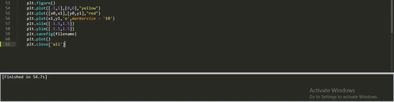
While executing programming code an error occured for the memory storages of those 200 images.

These error can be cleared by using plt.close('all') . This will erase all the memory of the images stored which results in finishing the code earlier.

The video animation is attached as youtube link.

https://youtu.be/vGb_XFAvzJw

Reference :

https://www.acs.psu.edu/drussell/Demos/Pendulum/Pendulum.html

https://ximera.osu.edu/ode/main/simplePendulum/simplePendulum