Week 3 - Solving second order ODEs

Objective:

To write a program that solves the ODE that represents the equation of a motion of a simple pendulum with damping. And also, to simulate the transient behavior of a simple pendulum and to create an animation of its motion.

Problem Statement:

In Engineering, ODE is used to describe the transient behaviour of a system. A simple example is a pendulum. The way the pendulum moves depends on the Newtons second law. When this law is written down, we get a second order Ordinary Differential Equation that describes the position of the "ball" w.r.t time.

A simple pendulum consists of a mass m hanging from a string of length L and fixed at a pivot point. When displaced to an initial angle and released, the pendulum will swing back and forth with periodic motion. By applying Newton's second law for rotational systems, the equation of motion for the pendulum may be obtained

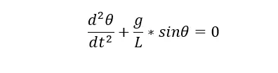
The primary forces acting on the bob are the gravitational force that makes it move in the first place and the force exerted by the string to keep it moving along a circular path. In addition, there may be a damping force from friction at the pivot or air resistance or both.

Assuming that the damping force is proportional to velocity. Since arc length and central angle are themselves proportional (with proportionality constant. The negative sign is because the damping force has to be opposite the direction of motion. When this term is included in the model, the equation becomes:

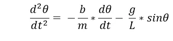
In the above equation,

g = gravity in m/s²,

L = length of the pendulum in m,

m = mass of the ball in kg,

b=damping coefficient.

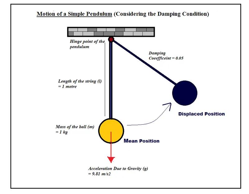
Given values for the parameters:

1. L=1 metre,
2. m=1 kg,
3. b=0.05.
4. g=9.81 m/s2.
5. Time period to be considered 0-20 sec,
6. angular displacement=0, angular velocity=3 rad/sec at time t=0.

Code:

clear all
close all
clc

%inputs
%length of the pendulum in m
l=1;
%mass of the ball in kg
m=1;
%damping coeffiecient
b=0.05;
%gravity in m/s2
g=9.81;

%Initial Conditions
%Angular displacement
theta_0=[0;3];
%angular velocity
omega_0=3;

%time_cordinates
t_span=linspace(0,20,500); %observing the motion for 20 secs

%ODE solver
[t, results]=ode45(@(t, theta) ode_func(t,theta,b,g,l,m),t_span,[0 3]);

figure(1)
%plotting angular displacement
A=plot(t,results(:,1));
legend([A], 'Angular Displacement');
hold on
%plotting angular velocity
B=plot(t, results(:,2));
legend([B], 'Angular Displacement');
ylabel('Plot')
xlabel('Time(seconds)')
hold off

displacement=results(:,1);
velocity=results(:,2);
x_start=1;
y_start=1;
ct=1;
for i=1:length(displacement)
    
    x_end=1-l*sin(displacement(i));
    y_end=1-l*cos(displacement(i));
    
    figure(2)
    %plot fixed link
    plot([0 2],[1 1],'linewidth',15,'color','b')
    hold on
    plot([1 x_end], [1 y_end], [x_end x_end], [y_end y_end], '-O', 'markersize', 15, 'markerfacecolor', 'r', 'linewidth',4)
    plot(x_start,y_start,'-O', 'markersize', 3, 'markerfacecolor', 'b')
    %axis setting
    axis([0 2 -0.5 2])
    
    M(ct)=getframe(gcf);
    ct=ct+1;
    hold off
end
movie(M)
videofile= VideoWriter('Simple pendulum.avi', 'uncompressed AVI');
open(videofile)
writeVideo(videofile, M)
close(videofile)

function[dtheta_dt]=ode_func(t,theta,b,g,l,m)
theta1=theta(1);
theta2=theta(2);

dtheta1_dt=theta2;
dtheta2_dt=-(b/m)*theta2-(g/l)*sin(theta1);
dtheta_dt=[dtheta1_dt;dtheta2_dt];
end

Result:

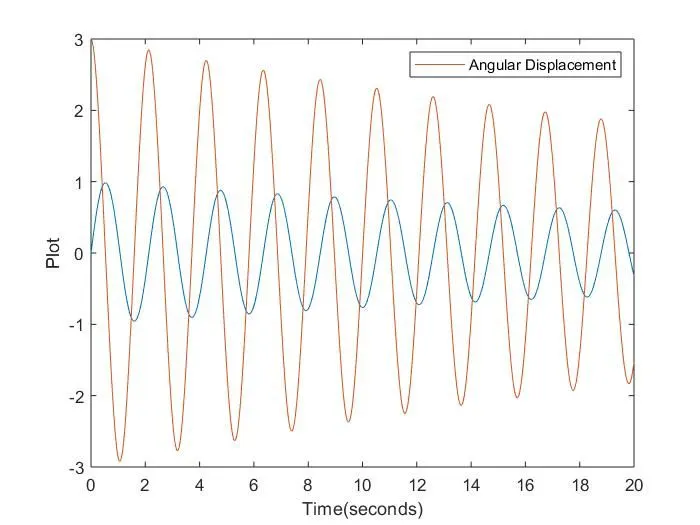
Plots are formed for Angular Displacement, Angular Velocity with respect to Time.

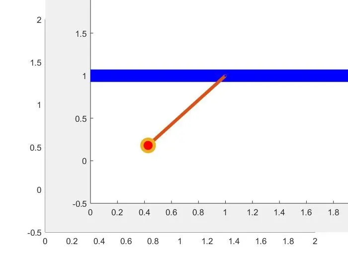
Link:

https://youtu.be/H2zcA_WEe_w

Discussion:

In a vacuum with zero air resistance, a pendulum will continue to oscillate indefinitely with a constant amplitude. However, the amplitude of a simple pendulum oscillating in the air continuously decreases as its mechanical energy is gradually lost due to air resistance.