Week 3 - Solving second order ODEs

Simple pendulum:

A simple pendulum is one that can be considered to be a point mass suspended from a string or rod of negligible mass. It is a resonant system with a single resonant frequency. Pendulum, body suspended from a fixed point so that it can swing back and forth under the influence of gravity. These are used to regulate the movement of clocks because of the interval of time for each complete oscillation. The time taken by a simple pendulum to complete the one complete oscillation is known as the Time period of a simple pendulum. 

                                      

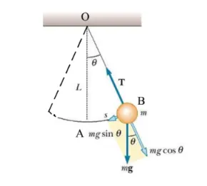
Given equation

`(d^2theta)/(dt)^2 + (b/m)((d theta)/dt) + (gsintheta)/l = 0`

we assume that 

1. `theta = theta_1`

2. `(d theta)/(dt) = (d theta_1)/(dt) = theta_2`

3. Now from the above equations we can written as `(d^2 theta)/(dt^2) = (d theta_2)/(dt)`

Substituting the above 3 equations in the given equation, we get

4. `(d theta_2)/(dt) = -(b/m)theta_2 - (g/l)sintheta_1`

we are mentioned these 4 equations in the functions code.

Given inputs:

Length of the pendulum(L) = 1m; 

Damping coefficient(b) = 0.05; 

Mass of the ball(m) = 1kg; 

Gravity(g) = 9.81 `m/s^2`,

Time(t) = 0, 

Angular displacement = 0;

Angular velocity = 3 rad/sec.

Code:-

# Second order ODE 

import math  # for doing mathamatical calculations
import matplotlib.pyplot as plt  # for ploting
import numpy as np # numpy is used to +, -, *, /, power, and linspace for the arrays
from scipy.integrate import odeint

# function
def model(theta,t,b,g,l,m):
	theta1 = theta[0]
	theta2 = theta[1]
	dtheta1_dt = theta2
	dtheta2_dt = -(b/m)*theta2-(g/l)*math.sin(theta1)
	dtheta_dt = [dtheta1_dt,dtheta2_dt]
	return dtheta_dt 

# inputs
b = 0.05
l = 1
m = 0.1
g = 9.81

# initial equation
theta_0 = [math.pi/2,0]

# time points
t = np.linspace(0,10,150)

# solve ODE
theta = odeint(model,theta_0,t,args=(b,g,l,m))

# plot results
plt.plot(t,theta[:,0],'b-',label=r'$\frac{d\theta_1}{dt}=\theta_2$')  # time Vs displacement 
plt.plot(t,theta[:,1],'r--',label=r'$\frac{d\theta2}{dt}=-\frac{b}{m}\theta_2 - \frac{g}{l}sin\theta_1$')  # time Vs velocity
plt.xlabel('time')
plt.ylabel('displacement, velocity')
plt.legend(loc='best')
plt.show()

val = theta[:,0]
ct  = 1
for i in range(0,len(val)):
	plt.figure()
	x1 = 0.5 - l*np.sin(val[i])
	y1 = 0.5 - l*np.cos(val[i])
	plt.plot([0.5,x1],[0.5,y1])
	plt.plot(x1,y1,'o',markersize = 8)
	plt.plot([-0.8,1.8],[0.5,0.5],linewidth = 2)
	plt.xlim([-0.8,1.8])
	plt.ylim([-0.8,0.6])
	filename = str(ct) + '.png'
	plt.savefig(filename)
	ct = ct+1

Result:-

 

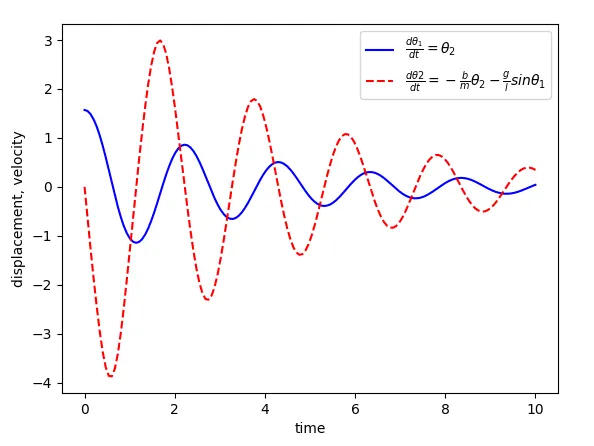
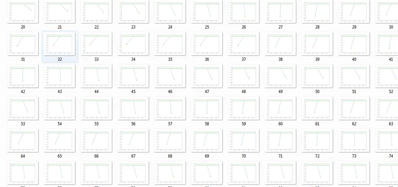
Animation link:-

All images are copied in Imgflip.com to create the simple pendulum animation. The animation link was given below:

 file:///E:/Skill%20lync/Python%20&%20cantera/simple%20pendulum/simple%20pendulum.gif