Python for Mechanical Engineers

Week 3 - Solving second order ODEs

Objective: To write a program to simulate the transient behaviour of a simple pendulum and to create an animation of its motion

Theory:

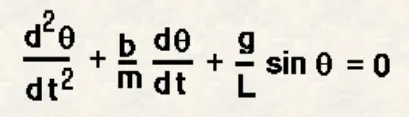
This is the second order ODE given to us for damped oscillatory motion of a simple pendulum

where, g=gravity in m/s^2

L=length of the pendulum in m

m=mass of the ball in kg

b= damping coefficient

Now for solving the second order ODE, we will first convert this second order ODE into a number of first order ODEs.

we will write a separate function where we will assume two variables theta1 and theta2, where theta2 is the first order differential of theta1 and

theta2=theta.Now using the equation given we will make an equation for theta2 where, theta2=-b/m*theta1-g/l*sin(theta1)

Main program:

import math
import numpy as np 
import matplotlib.pyplot as plt 
from scipy.integrate import odeint

def model(theta,t,b,g,l,m):
	theta1 = theta[0]
	theta2 = theta[1]

	dtheta1_dt = theta2
	dtheta2_dt = -(b/m) * theta2 - (g/l) * math.sin(theta1)
	return [dtheta1_dt, dtheta2_dt]

b = 0.05
g = 9.81
l = 1.0
m = 2

theta0 = [0, 5]

t = np.linspace(0,10,150)

k = odeint(model,theta0,t,args=(b,g,l,m))

#Plot results
plt.plot(t,k[:,0],'g' ,label=r'displacement') # g -> green 
plt.plot(t,k[:,1],'b' ,label=r'velocity') # b -> blue
plt.xlabel('plot')
plt.ylabel('Time')
plt.legend()
plt.savefig('output.png')
plt.show()

'''
a = k[:,0]
b = k[:,1]
'''
# Animation
ct = 1

for i in k[:,0]:
	x0 = 0
	y0 = 0

	x1 = l * (math.sin(i))                
	y1 = -l * (math.cos(i))   # using sin and cos function to locate the cordinates of #mass

	filename = str(ct) + '.png'
	ct = ct + 1
	plt.figure()
	plt.plot([-0.5,0.5],[0,0])  # horizontal support
	plt.plot([x0,x1],[y0,y1])   # pendulum string by connecting 2 points
	plt.plot(x1,y1,marker='.',markersize=20)# x1 , y1 = center of mass / pendulum #representation !
	plt.xlim([-1.5,1.5])
	plt.ylim([-1.5,1.5])
	plt.savefig(filename)

Explanation of code:

Initially we are importing required modules using 'import' command.

Function model is created with required arguments, inside which the term which are broken to solve second order ODE are calculated.

Inputs are provided for the function.

theta_0 ranges between 0 to 5.

odeint command is used to solve ode function.

Then results are plotted using plotting command.

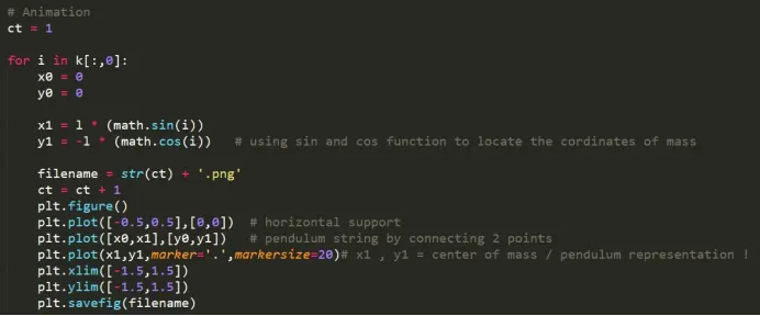
For creating animation we open a for loop

Images are saved using savefig command.

Output screenshot:

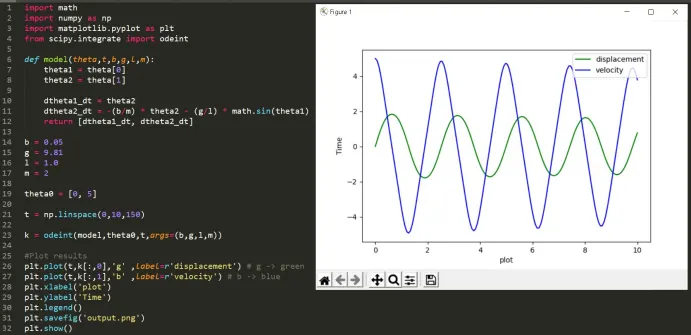
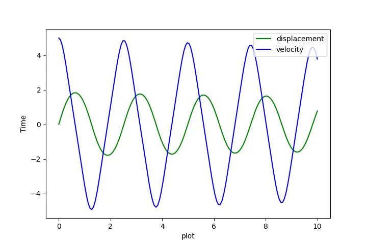
Conclusion : from the graph it can be seen that the values of angular displacement and angular velocity keeps on decreasing with time , this effect is know as

damping effect.

Errors :

Basic syntax errors are made during fifirst attempt, those are sooner rectifified and corrected

Animation link :

Simple Pendulum

-FFmpeg software is used to generate the video from the pictures using the following command in the command prompt.

ffmpeg -i %d.png Simple_Pendulum.avi

-Use the command only after getting into the parent folder where all the images have been saved in proper sequence.