Week 3 - Solving second order ODEs

Aim:To write a Matlab code to solve an Ordinary Differential Equation (ODE) which represents equation of motion of a simple pendulum and simulate the same.

Governing Equations:

In this case of Simple Pendulum Newton’s Second law is used.

The ODE that define the equation of motion of the pendulum is,

`(d^2theta)/dt^2 +(b/m)*(d theta)/dt+(g/l)*sintheta = 0` _____________ (1)

In above equation,

`theta`= angular displacement,

g = acceleration due to gravity in m/`s^2`,

l = length of the pendulum in meter,

m = mass of the bob in kg,

b=damping coefficient.

Above equation is 2^nd order ODE as it has `(d^2theta)/dt^2` and for solving this 2^nd order ODE , we should break it into two different 1^st order ODE so that it will easy for us to write the code in Matlab. For this following steps are taken into consideration.

`theta = theta_1` _________ (2)

This will result

`(d theta)/dt=(d theta_1)/dt`

`(d theta_1)/dt=theta_2` _________ (3)

So

`(d^2 theta)/dt^2=(d^2 theta_1)/dt^2=d/dt((d theta_1)/dt)=(d theta_2)/dt` _____ (4)

And all together we will get from above equations following equations

`(d^2theta_1)/dt^2 +(b/m)*(d theta_1)/dt+(g/l)*sintheta_1 =0`

And

`(d theta_2)/dt+(b/m)*theta_2 +(g/l)*sin theta_1 =0`

Thus

`(d theta_2)/dt=-(b/m)*theta_2 -(g/l)*sin theta_1` __________(5)

Thus we get two first order equation and these two ODEs can be represented in the matrix form to enter into MATLAB code.

`d/dt [(theta_1), (theta_2)] = [(theta_2), ((-b/m)*theta2-(g/l)*sintheta_1)]`

These ODEs are solved by ode45 and I will explain it in later part of this project.

In order to find the co-ordinates of the two ends of pendulum I used trigonometric relation

As we know that one end of the pendulum is fixed to a fixed surface, so its co-ordinate values are also constant, let’s say (0,0) and for this x₀ and y₀ coordinates are assigned.

The co-ordinates of the other end of the pendulum considered as (`x_1,y_1`) and they are calculated using following equations,

`x_1 = l*sin(theta)` _______ (6)

`y_1= -l*cos(theta)` ________(7)

In above equations `l` = length of string

`theta` = angular displacement

These are the governing equations used in the code.

OBJECTIVE:

1. To solve the 2nd order ODE by using MATLAB and find the values of angular displacement (i.e. `theta`) and angular velocity at different time span of the pendulum.
2. To create an animation video representing the motion of the pendulum.

Program

clear all
close all
clc

b = 0.05;
g=9.81;
m=1;
l=1;

%Initial conditions
theta_0 = [0;3];


%time points
t_span = linspace(0,20,500);

%solve ODE
[t,results] = ode45(@(t,theta)ode_func(t,theta,b,g,l,m),t_span,theta_0);

plot(t,results(:,1));
hold on
plot(t,results(:,2));
ylabel('Plot');
xlabel('time');
legend('Displacement','Velocity')



%animation 
ct = 1; 
for i = 1:length(t_span); %for loop used here with i renging from 1 to 500
 figure(2) % new figure to capture frames 
 
 x0 = 0; % x coordiante of fixed point of the pendulum
 y0 = 0; % y coordiante of fixed point of the pendulum
 x1 = l*sin(results(i,1)); % x coordiante of the end point of the pendulum
 y1 = -l*cos(results(i,1)); % y coordiante of the end point of the pendulum
  
 plot([-2 3],[0 0],'linewidth',2 ); % fixed line as the support of the pendulum 
 hold on
 plot([x0 x1],[y0 y1],'linewidth',2); % line connecting fixed point to end point 
 plot(x1,y1,'O','markersize',15); % ball of the pendulum
 hold off 
 axis([-1.5 1.5 -1.5 1.5]); %axis
 pause(0.03);
 M(ct)=getframe(gcf);
 ct = ct+1;
end
 movie(M)
videofile = VideoWriter('ode.avi','Uncompressed AVI')
open(videofile)
writeVideo(videofile,M)
close(videofile)
    

EXPLANATION:

clear all

close all

clc

The code is started with ‘close all’, ‘clear all’, ‘clc’ to close any previous plots, workspace and command window.

b = 0.05;

g=9.81;

m=1;

l=1;

The inputs are entered i.e. damping coefficient (b), acceleration due to gravity (g),mass of the bob (m) and length of the pendulum (l).

%Initial conditions

theta_0 = [0;3];

Then the initial conditions i.e. initial angular displacement [0] and initial angular velocity of the pendulum [3] are given as inputs values as a column vector because the 2^nd order ODE we have broken into two 1^st order ODEs which are representing angular displacement (3) and angular velocity (5).

%time points

t_span = linspace(0,20,500);

Above command represents the time interval up-to which the motion of the pendulum must be calculated. Here the time interval is taken from 0-20 seconds with 500 values between them.

%solve ODE

[t,results] = ode45(@(t,theta)ode_func(t,theta,b,g,l,m),t_span,theta_0);

Then to solve the ODE, I have used a command called ‘ode45()’ which is in-built Matlab solver.

The function ode45 takes 3 inputs. The 3 inputs are the function to be integrated, the time span and the initial conditions.

[t,results] = ode45(@(t,theta)ode_func(t,theta,b,g,l,m),t_span,theta_0);

Here,

[t , results] is solution vector and Matlab returns results for each time t.

func(t,theta,b,g,l,m) is the function for ODE

theta_0 is initial conditions representing.

t_span is final value until which solution is desired.

The ODE defined in our problem is dependent on ‘t’ and ‘θ’ we have enter as ‘@(t,theta)' .

A function is defined separately with the inputs and then it is used in ‘ode45’ command.

ODE45 Function

function[dtheta_dt] = ode_func(t,theta,b,g,l,m)

    theta1 = theta(1);
    theta2 = theta(2);
    dtheta1_dt = theta2;
    dtheta2_dt = -(b/m)*theta2 - (g/l)*sin(theta1);
    dtheta_dt = [dtheta1_dt;dtheta2_dt];
end

The ODE defined in our problem is dependent on ‘t’ and ‘θ’ we have enter as ‘@(t,theta)' .

A function is defined separately with the inputs and then it is used in ‘ode45’ command.

In the above function entered we have used the equations (2), (3), (4) ,(5) and the matrix which was derived above.

function[dtheta_dt] = ode_func(t,theta,b,g,l,m)

The function name is given as ‘ode_func’ and the inputs for this function are given as time (t), angular displacement theta, damping coefficient (b), acceleration due to gravity (g), length of the pendulum (l), mass of the bob (m).

dtheta1_dt = theta2;

dtheta2_dt = -(b/m)*theta2 - (g/l)*sin(theta1)

Above two equations represent the two values of `theta_1` and `theta_2`

dtheta_dt = [dtheta1_dt;dtheta2_dt];

This will create the matrix with two columns.

Now this function is saved in the same folder where the main code is saved and then this function is called in the 'ode45' command.

[t,results] = ode45(@(t,theta)ode_func(t,theta,b,g,l,m),t_span,theta_0);

Since initial and final time is defined as t_span so it is entered directly in the ‘ode45’ command, and similarly initial conditions are defined in the variable theta_0

After execution of the code we will get 500 values for ‘t’ and for ‘results’ a (500x2) matrix.

In the results the first column represents the values of angular displacements and second column represents values of angular velocities

plot(t,results(:,1));

hold on

plot(t,results(:,2));

ylabel('Plot');

xlabel('time');

To obtain a graph we have above command. First ‘plot()’ is used for generating a curve that represents how angular displacement changes with time and second ‘plot()’ command is used to generate a curve that represents how angular velocity changes with time. Then 'legend()' command is used to show which curve represents angular displacement and ngular velocity in the graph.

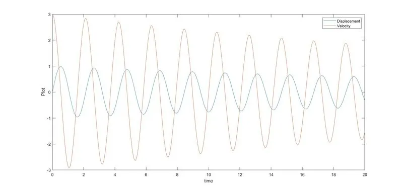
ANIMATION

To create an animation video need to track different positions of the pendulum at each time interval.

Position of the pendulum is determined by the values of angular displacement.

As we know first column of the ‘results’ matrix are the values of displacement and we can use those.

For Loop is used to determine the different positions of the pendulum.

In this loop value of i is taken as ‘i=1: 1:length(t_span)’, which means that ‘i’ will vary from 1 to last time span that is 500 .

x0 = 0; % x coordiante of fixed point of the pendulum

y0 = 0; % y coordiante of fixed point of the pendulum

x1 = l*sin(results(i,1)); % x coordiante of the end point of the pendulum

y1 = -l*cos(results(i,1)); % y coordiante of the end point of the pendulum

Next fixed end point of the pendulum is defined i.e. ‘x0’, ‘y0’, at (0,0)

Then the other end points of the pendulum are defined using the equation(6) and equation(7) as mentioned above.

plot([-2 3],[0 0],'linewidth',2 );

This is for drawing fixed line as the support of the pendulum

hold on

plot([x0 x1],[y0 y1],'linewidth',2);

This is for line connecting fixed point to end point

plot(x1,y1,'O','markersize',15);

To draw a ball of the pendulum

hold off

axis([-1.5 1.5 -1.5 1.5]);

This will define axis

pause(0.03);

M(ct)=getframe(gcf);

It will store the frames.

ct = ct+1;

Ct value is added by 1

This complets For Loop

M(ct)=getframe(gcf);

The command getframe(gcf); captures the entire interior of the current figure window i.e. get current figure and it will be assigned to an array M(ct).

Then movie(M) command will generate movie with all the frames.

videofile = Videowiter('ode.avi','Uncompressed AVI'); will create videofile

open(videofile) will open this video file then I use writeideo(videofile,M) command to write the video file and inside that write the frames which are captured in M. Lastly close the video file by close(videofile) command.

ERROS:

No serious error occured this time. Typo erros need not to be listed.

CONCLUSIONS:

Thus with the code given above we we can solve the ODE to equation of motion of a simple pendulum and created a animated video of the pendulum successfully.