Week 3 - Solving second order ODEs
CREATING MOVIE OF SIMPLE PENDULUM IN MATLAB BY SOLVING 2ND ORDER ODE
OBJECTIVE:
- To write a program that solves the following ODE. The ODE below represents the equation of motion of a simple pendulum with damping.
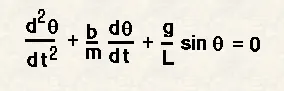
- Write a program in MATLAB that will simulate the pendulum motion, just like the one shown below.
- Simulate the motion between 0-20 sec, for angular displacement=0, angular velocity=3 rad/sec at time t=0. When you do this, you will get the position of the pendulum as a function of time. Use this information to animate the motion of the pendulum, as shown in the below figure
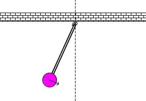
- The main aim is to simulate the transient behavior of Simple Pendulum and Create a movie using all the information.
INTRODUCTION:
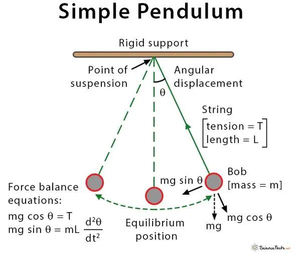
- A pendulum is a body suspended from a fixed support so that it swings freely back and forth under the influence of gravity. When a pendulum is displaced sideways from its resting, equilibrium position, it is subject to a restoring force due to gravity that will accelerate it back toward the equilibrium position. When released, the restoring force acting on the pendulum's mass causes it to oscillate about the equilibrium position, swinging it back and forth. The mathematics of pendulums is in general quite complicated. Simplifying assumptions can be made, which in the case of a simple pendulum allow the equations of motion to be solved analytically for small-angle oscillations.
- In mathematics, an ordinary differential equation (ODE) is a differential equation containing one or more functions of one independent variable and the derivatives of those functions. The term ordinary is used in contrast with the term partial differential equation which may be with respect to more than one independent variable.
REQUIRED EQUATIONS AND PRE-DEFINED FUNCTIONS:
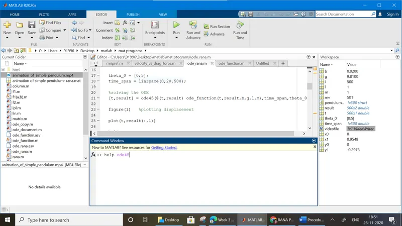
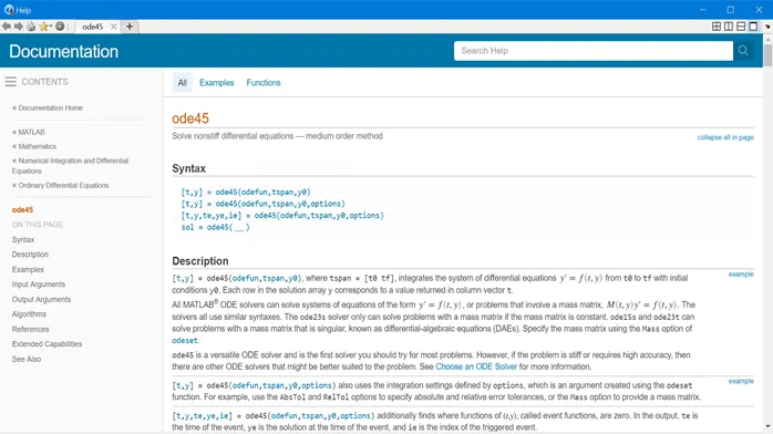
- In MATLAB if we want to see the documentation, examples about pre-defined functions, we have to type help “name of pre-defined” function. Then a documentation will be opened. This process is shown below.
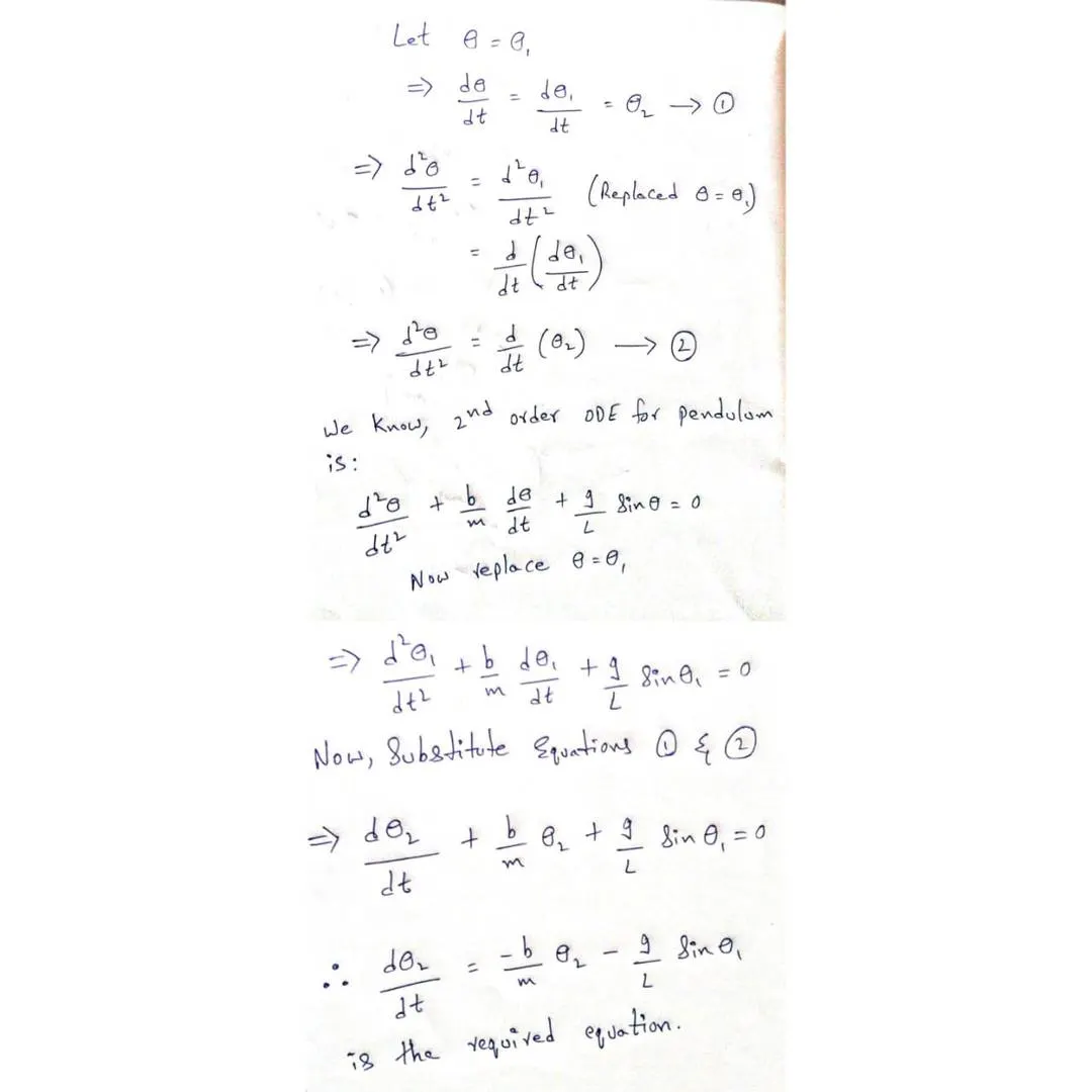
- I have derived the 2nd order ODE into 1st order ODE in the image below.
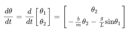
- If we arrange the above equation in matrix form we get,
Procedure:
- When we have 2nd order ODE, we must break it down into a set of 1st order ODE’s. Here, there are two 1st order Ode’s, they are -
- Displacement
- Velocity
- Now, the initial displacement & velocity values are assumed to be 0 & 5.
- To get a solution we need to integrate the equation.
- Integration is done within certain limits. We need to define these limits. This integration is done by “ODE45”, which is pre-defined MATLAB function.
- I have defined time span using ‘linspace’ command.
- Here, ‘t’ & ‘t_span’ are different. ‘t’ is the integration time & ‘t_span’ is a time array that has 500 values between 0 & 10.
theta_0 = [0;5];
time_span = linspace(0,20,500);
7. Now, I have created a function which inputs Damping Coefficient(b), force of gravity(g), mass of the bob(m), and length(l).
b = 0.02; %c = damping coefficient
g = 9.81; %g = force of gravity
m = 1;    %m = mass of bob
l = 1;    %l = length
8. Through “ode_function”, dtheta_dt is obtained. If you check output of ‘result’ in workspace, two columns will be formed which shows displacement and velocity.
%Function for calculating dtheta_dt

function [dtheta_dt] = ode_function(t,theta,b,g,l,m)

theta1 = theta(1);

theta2 = theta(2);

%to solve it easily we break down the 2nd order ODE to two 1st order ODE

%for displacement

dtheta1_dt = theta2;

%for angular velocity

dtheta2_dt = -(b/m)*theta2 - (g/l)*sin(theta1);

%final solution vector

dtheta_dt = [dtheta1_dt;dtheta2_dt];

end
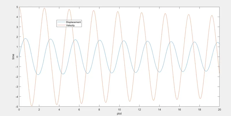
9. I have used ‘plot’ command to generate graph for angular displacement and angular velocity with respect to time.
10. For showing different position of the pendulum at different times, I have used ‘for loop’
11. By using ‘for loop’ & incrementing the value during each iteration.
12. Now, each iteration is plotted which creates individual frames of images.
13. By using hold ON/OFF, we can allow multiple plots to be drawn in same axes.
for i = 1:length(time_span)

    x1 = l*sin(result(i,1));

    y1 = -l*cos(result(i,1));

    %plotting the result

    figure(2)

    plot([x0,x1],[y0,y1],[-1,1],[0,0],'r-','linewidth',4,'markersize',10)

    hold on;

    plot(x1,y1,'marker','.','markerfacecolor','m','markersize',100)

    axis([-1.5 2 -1.5 2])

    hold off;

 pendulum_movie(mv) = getframe(gcf);

   mv = mv+1;

   pause(0.0004);

end
14. Select the colour, line width, market size & a symbol to represent the bob of the pendulum.
15. I have used “full stop” (.), and gave marker size as 100. This gave my animation a pendulum like structure.
16. After creating individual frames, I have used ‘get frame’ command which gathers all the individual frames and assigned it to a variable called pendulum_movie.
17. Therefore, a movie (or) animation is created under pendulum_movie.
18. Now we must save the movie.
19. For saving the movie we need to call ‘video writer’ which has file name and format (AVI, MPEG_4, etc.).
20. Now, I have assigned the ‘video writer’ to a video file.
21. At last we need to open the ‘video writer’, write the video and close the file.
movie(pendulum_movie)
videofile = VideoWriter('animation_of_simple_pendulum','mpeg-4');
videofile.FrameRate = 50;
open(videofile)
writeVideo(videofile , pendulum_movie)
close(videofile)
MAIN CODE:
clear all;

close all;

clc;

%inputs for ODE

b = 0.02; %c = damping coefficient

g = 9.81; %g = force of gravity

m = 1; %m = mass of bob

l = 1; %l = length

theta_0 = [0;5];
time_span = linspace(0,20,500);

%solving the ODE
[t,result] = ode45(@(t,result) ode_function(t,result,b,g,l,m),time_span,theta_0);

figure(1)   %plotting displacement

plot(t,result(:,1))

hold on;

plot(t,result(:,2))    %plotting velocity

xlabel('plot')

ylabel('time')

legend('Displacement','Velocity','location','best')


x0=0;
y0=0;
mv = 1;

%for loop for capturing different time frames
for i = 1:length(time_span)

    x1 = l*sin(result(i,1));

    y1 = -l*cos(result(i,1));

    %plotting the result

    figure(2)

    plot([x0,x1],[y0,y1],[-1,1],[0,0],'r-','linewidth',4,'markersize',10)

    hold on;

    plot(x1,y1,'marker','.','markerfacecolor','m','markersize',100)

    axis([-1.5 2 -1.5 2])

    hold off;

 pendulum_movie(mv) = getframe(gcf);

   mv = mv+1;

   pause(0.0004);

end

%Creating movie by using all the captured frames.

movie(pendulum_movie)

%here i have used MP4 format for saving the animation or movie
%we can use any type of format according to our usuage

videofile = VideoWriter('animation_of_simple_pendulum','mpeg-4');

%i have also provided framerate as 50 per second
videofile.FrameRate = 50;
open(videofile)
writeVideo(videofile , pendulum_movie)
close(videofile)
OUTPUT:
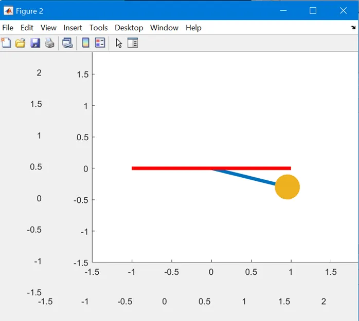
VIDEO LINK: https://youtu.be/8jpT3OxKZeQ