Week 3 - Solving second order ODEs

Aim

To create a code in sublime using python that solves the ordinary differential equation which represents the equation of the motion of a pendulum with damping along with the animation of the motion of the pendulum.

Algorithm

1. Solve the given ODE into two equations by introducing two new variables theta 1 and theta 2.
2. Now provide the initial conditions for the problem in the program like the time step, angular velocity, and angular displacement.
3. After the initial conditions are fixed provide the values of inputs under the constant section of the code like the value of gravity, the length of the pendulum, the mass of the pendulum, etc.
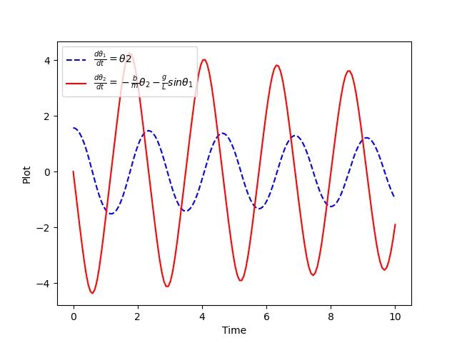
4. Now provide the commands for the plotting of the curve that shows the damping effect that is gradual dissipation of energy.
5. Now provide the code for the pendulum motion with the help of a straight line connected to a circle using the motions in sync with the results achieved by solving the differential equations.
6. Now install image magick software and then launch command prompt in windows or terminal if using linux or unix based operating system .
7. Now use the inbuilt command for movie generation so that the animation of the pendulum motion along with the graphs can be well captured and stored.

Python code

import math
import matplotlib.pyplot as plt
import numpy as np 
from scipy.integrate import odeint

# function which returns dz/dt
def model(theta,t,b,g,l,m):

	theta1=theta[0]
	theta2=theta[1]
	dtheta1_dt= theta2 # 1st generted ODE
	dtheta2_dt=-(b/m)*theta2-(g/l)*math.sin(theta1) #2nd generted ODE
	dtheta_dt=[dtheta1_dt,dtheta2_dt]
	return dtheta_dt # final value of the function

b=0.05 #damping coefficent
g=9.81 #acceleration due to gravity
l=1    #length of the pendulum
m=1  # mass of the pendulum

# Initial conditions
theta_0=[math.pi/2,0] # initial positon for the two odes generated from the original ode

# Time points

t=np.linspace(0,10,150)   # Integrating equation from t=0sec to t=10 sec by taking 150 points in between both the time values


#solve ODE
theta=odeint(model,theta_0,t,args=(b,g,l,m))# for solving the ode using the command within the scipy module using function definition, initial conditions ,time and arguments for ode


#plotting command

plt.plot(t,theta[:,0],'b--',Label=r'$\frac{d\theta_1}{dt}=\theta2$')
plt.plot(t,theta[:,1],'r-',Label=r'$\frac{d\theta_2}{dt}=-\frac{b}{m}\theta_2-\frac{g}{L}sin\theta_1$')
plt.ylabel('Plot')
plt.xlabel('Time')
plt.legend(loc='best')
plt.show()

# creating the animation of the pendulum

ct=1

for theta in theta[:,0]:
	x0=0
	y0=0 # the origin cordinates for the pendulum
	x1=1*math.sin(theta)
	y1=-1*math.cos(theta)
	plt.figure()
	plt.plot([-1,1],[0,0],"orange",linewidth=5)
	plt.plot([x0,x1],[y0,y1],"red")
	plt.plot(x1,y1,'o',markersize=20)
	plt.xlim([-2,2])
	plt.ylim([-1.5,1])
	ct=ct+1
	filename='sun%05d.png'%ct
	plt.savefig(filename)

Working of code

1. Firstly, import the python libraries required for this code to execute which are math, matplotlib, numpy and scipy which have various functions defined in them which will be used in this code.
2. Initial inputs such as length of the pendulum, the mass of the pendulum, damping coefficient, and acceleration due to gravity are defined in the code as per the question.
3. An array of initial theta was created to define initial angular displacement and initial angular velocity.
4. An array of time span was created to store 150 equally spaced intervals between time 0 to 10 seconds.
5. To solve the second-order ODE, a function named ode_function stores the above matrix data in it.
6. The given second-order ODE was solved using odeint command along with a proper syntax involving the calling of various functions resulting in the plotting of the graph between angular displacement and angular velocity with respect to time.
7. The last part of the code deals with the animation of the pendulum motion for which a loop was used and a counter variable was iterated inside the loop.
8. This animation makes sure that one of the strings of the pendulum is fixed while the other moves according to the solution of the ODE solved prior to the program.

Errors and solutions

• No major errors were found within the program expect syntax errors that were solved using the manual of the python.

Results

• The plot obtained by this program is given below

• An animation is generated in accordance with the motion of the pendulum obtained by solving the given ODE is uploded in youtube and its linnk is given below.

Conclusion

1. A python code is created in sublime that solves the ordinary differential equation which represents the equation of the motion of a pendulum with damping.
2. An animation is created capturing the motion of the pendulum along with damping which is obtained by solving the ODE.

Youtube link

https://youtu.be/byIKlNMQZYw