Simulating motion of simple pendulum by solving second order ODE

AIM:

To write a program to solve the second order Ordinary Differential Equation (ODE) representing the motion of a simple pendulum.

GOVERNMING EQUATIONS:

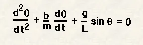
In the above equation, θ is the angle, t is the time span for integration. Damping co-efficient is represented by b, Mass of the pendulum (bob) by m, Acceleration due to gravity by g (9.81m/s²) and Length of the pendulum by l. The above equation represents the motion of simple pendulum when fixed from one end. Solving the above ODE, we will get the solution which can be used to get the motion of the pendulum in the form of a plot.

OBJECTIVE:

The objective of the project is to learn the working of for loop and create the plots representing the motion of a simple pendulum. Then combine all the plots together and create a video.

PROGRAMMING LANGUAGE USED:

MATLAB

CODE SAMPLE:

clear all
close all
clc

%Inputs

b = 0.05; %Damping co-efficient
g = 9.81; %Acceleration due to gravity (m/s2)
l = 1; %Length of pendulam (m)
m = 1; %Mass (kg)

%Initial condition
theta_0 = [0;3]; %Initial angular displacement is 0 and Initial angular velocity is 3 rad/s

t_span = linspace(0,20,400); %Time limit varying from 0 to 20 seconds

[t,results] = ode45(@(t,theta) ode_func(t,theta,b,g,l,m),t_span,theta_0);

figure(1)
plot(t,results(:,1),'linewidth',2)
hold on
plot(t,results(:,2),'linewidth',2)
legend('Angular displacement (rad)','Angular velocity(rad/sec)')
ylabel('Angular displacement / velocity →')
xlabel('Time (sec)→')
hold on 

ct = 1;

 x0 = 0;
 y0 = 4;

for i = 1:length(results(:,1))

THETA = results(i,1);
      
x1 = l*sin(THETA);
y1 = -l*cos(THETA);

figure(2)
plot([-5,5],[4,4],'color','black','linewidth',4); %Plotting base of the pendulum
hold on
plot([x0 x1],[y0 y1],'linewidth',3,'color','red'); %Plotting the string
hold on
plot(x1,y1,'marker','O','markersize',20,'markerfacecolor','blue'); %Plotting the bob
axis([-4 4,-4 4]); 
hold off
pause(0.03)
V(ct) = getframe(gcf);
ct = ct + 1;
end

%Creating a video of all the obtained plots in array V
movie(V);

%Naming the video file and its profile
videofile = VideoWriter('Simple pendulum simulation.avi','Uncompressed AVI');

open(videofile);

%Writing all the figures (plots) in array V into the video file
writeVideo(videofile,V);
close(videofile);

Function ode_func

function [dtheta_dt] = ode_func(t,theta,b,g,l,m)

theta1 = theta(1);
theta2 = theta(2);
dtheta1_dt = theta2;
dtheta2_dt = (-b/m)*theta2-(g/l)*sin(theta1);
dtheta_dt = [dtheta1_dt;dtheta2_dt];
end

ALGORITHM:

First the inputs required for the programming are defined. The damping co-efficient (b), acceleration due to gravity (g), length of pendulum (l) and mass of the pendulum (m) are defined and given values. The initial conditions for angular displacement and angular velocity along with time limit is also specified and defined.

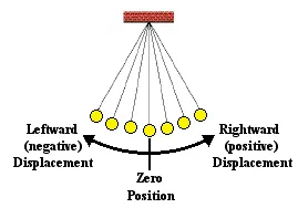
Then the solution for the equation, time and angular displacement & velocity are calculated using the ode45 solver in MATLAB by calling the function which is pre-defined. This function solves the second order ODE by reducing it into lower order ODEs. After the solutions are computed, they are plot on a graph. Then the position of the pendulum is depicted on a separate plot. The positions of the pendulum are all collected and combined into a video form by MATLAB and given as the output.

EXPLANATION:

Initially, the inputs for damping co-efficient, acceleration due to gravity, length and mass of the pendulum are given. The damping co-efficient is given as 0.05, acceleration due to gravity is given as 9.81 m/s², length of the pendulum (string) is given as 1m and mass as 1kg. They are stored in variables b, g, l and m. Then the initial condition variables, angular displacement & velocity are given as 0 and 3 and time as 0 to 20 seconds are given. They are also stored in variables theta_0 and time_span. The time span limit given is split in 400 using the linspace command.

Then the solution for the ODE is computed using the ode45 solver. ode45 is an inbuilt solver in MATLAB which is used to solve Ordinary Differential Equations. The t and theta values are unknown and this is also given as an input to the ode45 solver by adding the @ symbol. The values for b, g, l and m are given and substituted in the function ode_func. The output from the function and ode45 are stored in the output array [t,results]. In the output array, t stores the time values and results stores the angular displacement and velocity.

Then the obtained results are plot on a graph. The values for angular displacement and velocity are plot versus the time on a single graph. The motion of the pendulum is plot on a separate graph. This is done using the for loop. First, the fixed end of the pendulum is plot by fixing the co-ordinates for that point. Then the other end of the pendulum, where the bob is fixed is calculated. Then the base of the pendulum is plot by plotting a horizontal line of line-width 4 of black colour. Next the string for connecting the bob and the fixed end is plot. In between the two plot commands, a hold on command is used so that the earlier plots are not replaced by the subsequent plot command. Then the bob of the pendulum is plot and the axis for the plot is given. This graph is plot for every change in the angular displacement. Finally, a video of all the plots is created by combining the plots and the video is named accordingly.

ERRORS FACED:

While writing & executing the program, some errors faced are explained in detail below.

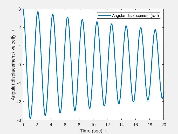
Here in the first plot we can see that there is only angular displacement. We find that angular displacement is missing. But the legend in the plot shows “Angular displacement”.

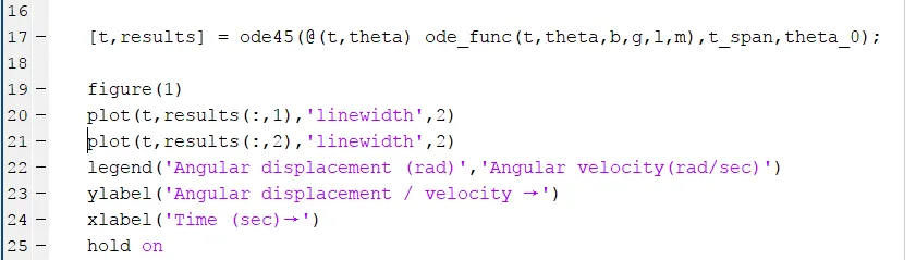
It is because we have missed to put the hold on command after the first plot command in line 21. As a result, the first plot depicting the angular displacement was replaced by the second plot depicting angular velocity. Hence the angular displacement is missing.

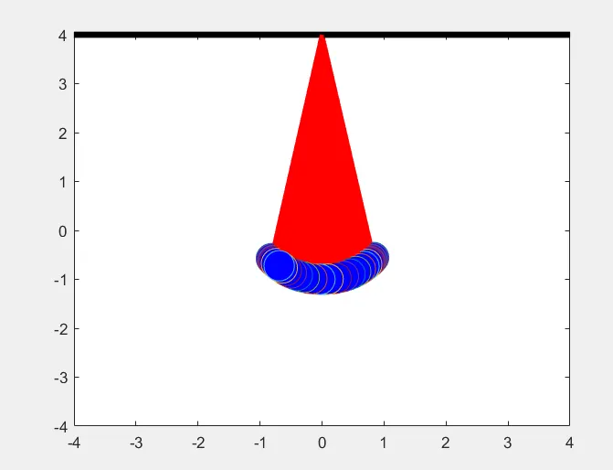
Here, we can see that the motion of the pendulum is recorded but the plot obtained is overlapping.

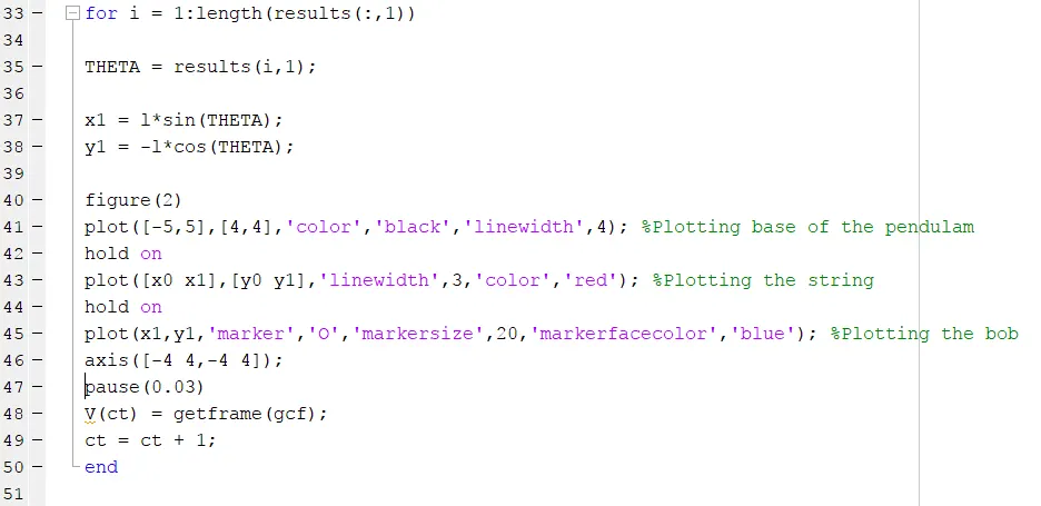
It is so because after giving the plot & hold on commands we have not given the hold off command which should be given in line 46. As a result, the plots are overlapping.

RESULTS:

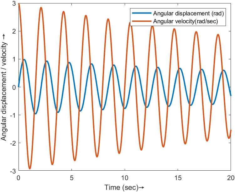
After the program is successfully executed, we will obtain the results. We can see the plot between angular displacement & velocity versus the time in one plot. Also, we have obtained a simulation of the motion of the pendulum with the solutions for the ODEs.

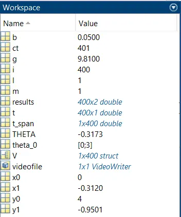
We can find the solutions and values of the variables in the workspace window. It shows the values of all the variables used in the program.

LEARNING OUTCOME:

From the above project, we have learnt the concept of using for loop, the need and its method of using. We have also learnt the method of using solver ode45 in MATLAB for solving Ordinary Differential Equations and creating video of all the plots.

CONCLUSION:

Thus the MATLAB program for depicting the motion of a simple pendulum is written which can be used to solve Ordinary Differential Equations.