Week 3 - Solving second order ODEs

AIM: To write a program to stimulate the transient behaviour of a simple pendulum and create an animation of its motion.

THEORY:

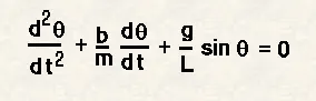
This is the second order ODE given to us for damped oscillatory motion of a simple pendulum

where,

g = gravity in m/s2,

L = length of the pendulum in m,

m = mass of the ball in kg,

b=damping coefficient.

OBJECTIVE:

To write a program in Python that will simulate the pendulum motion.

PROCEDURE:

#importing required modules

import math
from scipy.integrate import odeint
import matplotlib.pyplot as plt
import numpy as np

#function that returns dz/dt
from scipy.ndimage import label


def model(theta,t,b,g,l,m):

    theta1=theta[0]
    theta2=theta[1]
    dtheta1_dt=theta2
    dtheta2_dt=-(b/m)*theta2-(g/l)*math.sin(theta1)
    dtheta_dt=[dtheta1_dt,dtheta2_dt]
    return dtheta_dt

b=0.05
g=9.81
l=1
m=1

#initial condition
theta_0=[0,5]

#time points
t=np.linspace(0,20,200)

#solve ODE
theta=odeint(model,theta_0,t,args=(b,g,l,m))

#plot results
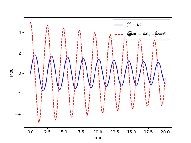
plt.plot(t,theta[:,0],'b-',label=r'$\frac{d\theta_1}{dt}=\theta2$')
plt.plot(t,theta[:,1],'r--',label=r'$\frac{d\theta2}{dt}=-\frac{b}{m}\theta_2-\frac{g}{L}sin\theta_1$')
plt.xlabel('time')
plt.ylabel('Plot')
plt.legend(loc='best')
plt.show()

#Animation step
ct=1
x0=5
y0=5
for i in range(len(t)):
    x1=x0+1*math.sin(theta[i,0])
    y1=y0-1*math.cos(theta[i,0])
    filename='pendulum'+str(ct)+'.png'



    plt.figure()
    plt.plot([4,6],[5,5],'k-')
    plt.plot([x0,x1],[y0,y1])
    plt.plot(x1,y1,marker='0',markersize='10')
    plt.axis([3.5,6.5,3,6])
    plt.savefig(filename)
    ct=ct+1
RESULT:

The simulation of the simple pendulum is given below in the link 
https://youtu.be/-jdlO--8jMU 
CONCLUSION:
The simulation of the simple pendulum was created using python program also the
 transient behaviour of pendulum was shown using the program.