Week 3 - Solving second order ODEs

Objective:

Write a program to simulate the transient behavior of a simple pendulum and to create an animation of its motion.

Theory:

In mathematics, an Ordinary Differential Equation (ODE) is a differential equation containing one or more functions of one independent variable and the derivatives of those functions.

In Engineering, ODE is used to describe the Transient Behaviour of the system.

Here, the motion of Simple Pendulum is also governing by Second Order ODE as below:-

import numpy as np
import matplotlib.pyplot as plt 
import math as mt 
from scipy.integrate import odeint

def model(theta,t,b,g,l,m):
   theta1=theta[0]
   theta2=theta[1]
   dtheta1_dt=theta2
   dtheta2_dt=-(b/m)*theta2-(g/l)*mt.sin(theta1)
   dtheta=[dtheta1_dt,dtheta2_dt]
   return dtheta
    
    
b=0.05
g=9.81
l=1
m=0.1
    
theta_0=[0,3]

t=np.linspace(0,50,150)

theta=odeint(model,theta_0,t,args=(b,g,l,m))
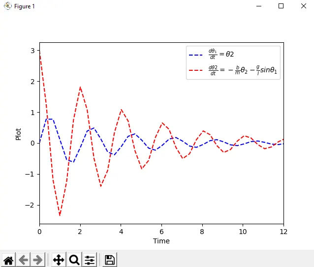
plt.plot(t,theta[:,0],'b--',label = r'$\frac{d\theta_1}{dt} = \theta2 $')
plt.plot(t,theta[:,1],'r--',label = r'$\frac{d\theta2}{dt} = -\frac{b}{m}\theta_2 -\frac{g}{l}sin\theta_1 $')
plt.xlabel('Time')
plt.ylabel('Plot')
plt.xlim([0,12])
plt.legend(loc = 'best')
plt.show()

ct=1                                #Counter Variable

for Theta in theta[:,0]:

	

	#Co-ordinates of Fixed Point of String

	x0 = 0

	y0 = 0

	#Co-ordinates of End Point of String

	x1 = l*mt.sin(Theta)

	y1 = -l*mt.cos(Theta)



	filename = str(ct) + '.png'

	ct = ct + 1



	plt.figure()

	#Plotting Horizontal Line

	plt.plot([-0.5,0.5],[0,0],'g',linewidth=5)

	#Plotting String of Pendulum

	plt.plot([x0,x1],[y0,y1],'r')

	#Plotting Ball of Pendulum

	plt.plot(x1,y1,'o',markersize=30)

	#Limiting X-axis

	plt.xlim([-1.5,1.5])

	#Limiting Y-axis

	plt.ylim([-1.5,1.5])

	#Title

	plt.title('Animation of Simple Pendulum using Python')

	#Saving Each Figure with its file name

	plt.savefig(filename)

output:

Animation file: