MATLAB: Solving second order differential equations (ODEs)

AIM

To solve an ordinary differential equation(ODE), that represents the equation of motion of a simple pendulum with damping.

OBJECTIVE

To simulate the pendulum motion using parameters, l being 1m, mass being 1kg, coefficient of daming being 0.05 and 9.81 being acceleration due to gravity, motion between 0-20s for angular velocity being 3 rad/s and angular displacement being 0 at time 0.

GOVERNING EQUATION

`(d^2theta)/dt^2+b/m*d/dt(theta)+g/l(sintheta)`

where, g = acceleration due to gravity

m = mass of the bob/ball

b = coefficient of damping

l = length of the string

theta = angular displacement

dtheta/dt= angular velocity

PROGRAM EXPLAINATION

1. Command was assigned to solve the ODE.

2. Clear all, close all and clc was assigned to clear out everything.

3. Now, all the parameters were specified in the editor window, along with their values.

4. Next, the initial conditions were initialised for velocity and displacement.

5. Now, t_span was given using linspace command.

6. The ODE was solved next calling the sub-function from another window that includes the values, parameters and the initial conditions. Along with these, it consists of needful matrix for further processing of plots.

7. Velocity and Position was plot next using the plot command along with leveling and other necessary commands.

8. Next, command for simulation was assigned and for loop was initiated with values for xo, yo, x1,y1.

9. Next, horizontal line for rigid surface was plot calling out the coordinates.

10. Similarly, Line was plot.

11. Next, marker was introduce to show the bob/ ball which was characterisied with the help of markerface and markercolour.

12. Now the frames in loop were arranged to form a movie as simulation for simple pendulum.

13. The program was saved, and was run. It did run successfully giving the required output.

PROGRAM CODE :

1. MAIN CODE

clear all
close all
clc

%damping coefficient
b = 0.05

%acceleration due to gravity (in m/s^2)
g = 9.81

%length of the pendulum (in m)
l = 1

%mass of th ball (in kg)
m = 1 

%initial condition
theta_0 = [0;3]

%time points
t_span = linspace(0,20,300)

%solve ODE
[t,results] = ode45(@(t,theta) ode_func(t,theta,b,g,l,m),t_span,theta_0);

    
hold on
%plotting displacement
plot(t,results(:,1))
%plotting velocity
plot(t,results(:,2))
xlabel('Time')
ylabel('Angular Velocity')
grid on

%simulation of motion of pendulum
ct=1
for i = 1:length(results(:,1))
    x0=0
    y0=0
    x1=l*sin(results(i,1))
    y1=-l*cos(results(i,1))
    
    
    %plotting horizontal line - RIGID SURFACE
    plot([-1 1],[0,0],'linewidth',3,'color','r')
    hold on
    %Plotting Axes
    plot([x0 x1],[y0 y1], 'linewidth',3,'color','g')
    axis([-2 2 -1.5 0.5])
    hold on
    plot(x1,y1,'marker', 'o','markersize',15,'markerfacecolor','b');
    hold off
    grid on 
    pause(0.03)    
    M(ct)= getframe(gcf)
    ct=ct+1
end
%creating animation/movie
movie(M)
videofile= VideoWriter('SimplePendulum.avi','uncompressed avi')
open(videofile)
writeVideo(videofile,M)
close(videofile)

2. SUBFUNCTION CODE

function [dtheta_dt] = ode_func(t,theta,b,g,l,m)
theta1=theta(1)
theta2=theta(2)
dtheta_1dt=theta2
dtheta_2dt=-((b/m)*theta2)-((g/l)*sin(theta1))
dtheta_dt = [dtheta_1dt;dtheta_2dt]
end

CHALLENGES FACED

1. The pendulum didn't run in X-Y Axis initially.

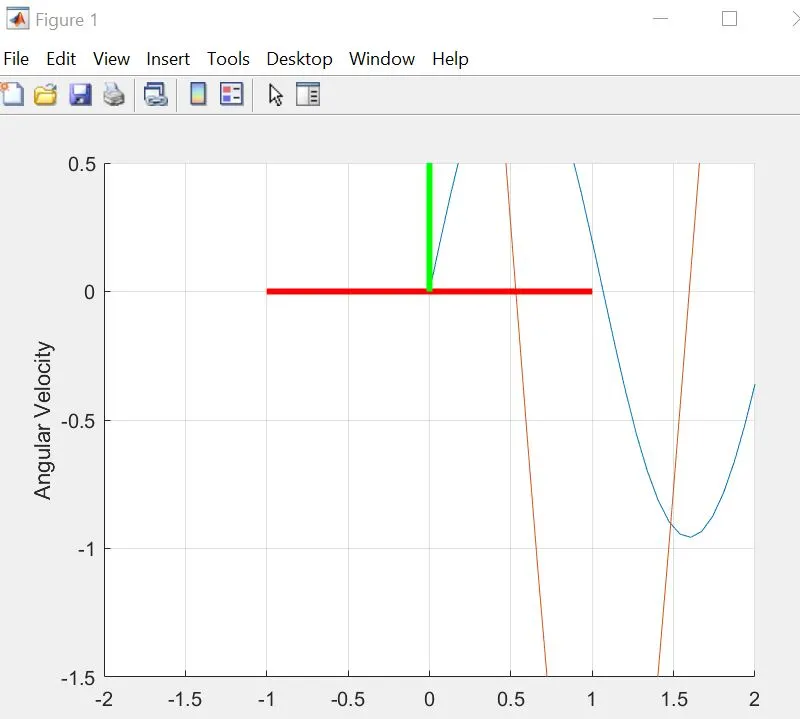
SOLUTION TO OVERCOME: Y1 value was changed from positive to negative.

2. Figure(1) was showing error after calling subfunction

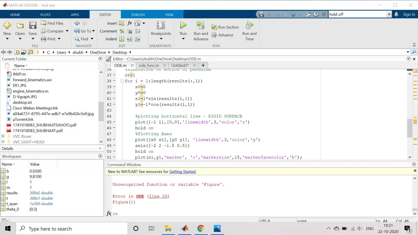
SOLUTION TO OVERCOME: Figure(1) was removed for successful run.

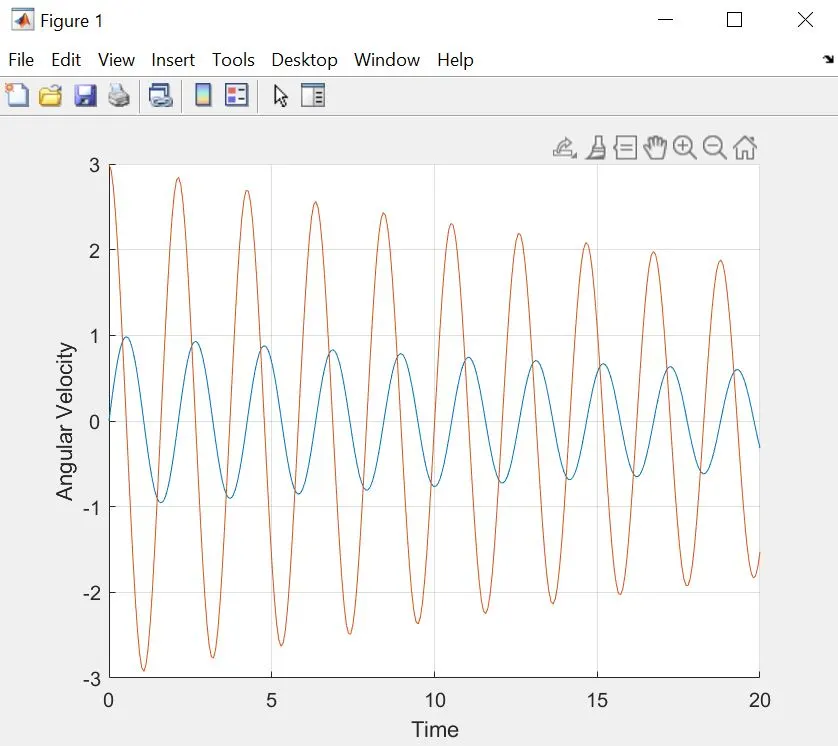
FIGURE SUPPORTING CONCLUSION

CONCLUSION

This ODE satisfies equation of motion for simple pendulum with damping and other required parameters. This draws conlusion that ODE describes the transient behaviour of a system.

ANIMATION SUPPORTING CONCLUSION

https://drive.google.com/file/d/14wHo2uovsRF4p8Gc-TgJ7LnMxbnWslty/view