Simulation of a Pendulum Oscillation using Second Order Differential Equation

Pendulum Oscillation using Second Order Differential Equation

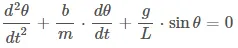
Aim: Creating a program in MATLAB to solve the following ODE and simulating the motion of a simple pendulum using ODE function.

Objective:

• To create a program to solve above Second ODE.

• To create a program in MATLAB that will simulate the pendulum motion.

Methodology:

Theory

The equation of motion of a simple pendulum is based on Newton second law of motion. A simple pendulum consists of a ball (point-mass) m hanging from a (massless) string of length L and fixed at a pivot point P.

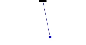
Fig: Oscillation of a Simple Pendulum.

The above is a motion of a simple pendulum. The motion of a pendulum can be defined as below by splitting bob motion into cosine and sine component.

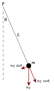
Fig: Splitting Bob motion in sine and cosine component.

As a result to find the position of bob at any given time is found out from the above.

When displaced to an initial angle and released, the pendulum will swing back and forth with periodic motion. By applying Newton's secont law for rotational systems, the equation of motion for the pendulum may be obtained.

which is;

Rearranging the equation;

The below equation is, second order differential equation of a simple damped pendulum:

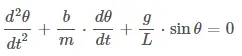
where,

b = damping coefficient(dimensionless)

m = mass(kg)

g = gravity(m/s²)

L = length of pendulum(m)

If the amplitude of angular displacement is small enough, so the small angle approximation holds true, then the equation of motion reduces to the equation of simple harmonic motion.

Lets assume;

..............................................................................(Equation 1)

We know that;

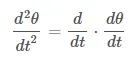
So,

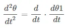
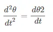
Replacing values;

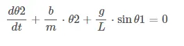
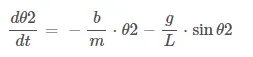............................................(Equation 2)

Rearranging equation 1 and 2 in matrix form.

......................................(Equation 3)

Program

Program to create an ode function

%Function for pendulum motion ode(Second ODE)
function [dtheta_dt] = pendode_func(time,theta,b,g,L,m)
theta1 = theta(1);                  %Displacement(rad)
theta2 = theta(2);                  %Velocity(rad/s)
dtheta1_dt = theta2;
dtheta2_dt = -(b/m)*theta2-(g/L)*sin(theta1);
dtheta_dt = [dtheta1_dt;dtheta2_dt];
end

In the above program, we have created a user-defined function for second ode of pendulum oscillation;

The name of the file is same as the name of funtion we will create.

The function that we have created is 'pendode_func' that will take values in the order (time,theta.b,g,L,m)

In variable 'theta1' the initial value of the displacament will be stored.

In variable 'theta2' the initial value of angular velocity will be stored.

Using equation 1 and equation 2, we will write the equation for 'dtheta1_dt' and 'dtheta2_dt'.

In equation 3, we have rearranged equation 1 and 2 in matrix form. Here too, we will do the same of assigning the equation in 'dtheta_dt'.

As the function equations are written and they are assigned to variable, we will close the function using 'end' command.

Program to plot 'Result v/s Time' and simulate 'Oscillation of a Pendulum'

%A program to plot the Pendulum motion (Second ODE)
clear all
close all
clc

%Input
b = 0.05;                %Damping(Dimensionless)
g = 9.81;                %Gravity(m/s^2)
L = 1;                   %Length(m)
m = 1;                   %Mass(kg)

%Initial Condition
theta_0 = [0;3];         %[angular displacement, angular velocity]

%Time Limit
timespan = linspace(0,20,500); %Creating 500 equally spaced timespan array between 0 and 20 sec

%Second ODE for pendulum 
[time,result] = ode45(@(time,theta) pendode_func(time,theta,b,g,L,m),timespan, theta_0);

%Plotting of Result v/s Time
figure(1)
plot(time,result(:,1),'--','color','r')
hold on
plot(time,result(:,2),'-.','color','b')
xlabel('Time(s)');
ylabel('[Displacement, Angular Velocity]');
title('Time v/s [Displacement, Angular Velocity]')
grid on
lgd = legend({'Displacement(rad)','Angular Velocity(rad/s)'},'Location','southeast');
title(lgd,'Damping');
legend('boxoff');

%Pendulum Motion;
ct = 1;                      %Initial Counter Value
for i = 1:length(result(:,1))
    %Hanging position of pendulum
    x0=0;
    y0=0;
    %Pendulum movement
    x1 = L*sin(result(i,1));
    y1 = -L*cos(result(i,1));
    %Pendulum Line
    figure(2)
    plot([x0,x1],[y0,y1],'Linewidth',2.5,'color','g'); 
    hold on
    %Pendulum Ball
    plot(x1,y1,'o','MarkerSize',15,'MarkerEdgeColor','b','MarkerFacecolor','r')
    %Hanging Line
    plot([-1,1],[0,0],'Linewidth',2,'color','c')
    legend('Pendulum String','Pendulum Bob','Hanging Line','FontSize',10,'TextColor','blue','NumColumns',2)
    legend('boxoff')
    %Hanging Point
    plot(x0,y0,'s','MarkerSize',7.5,'MarkerEdgeColor','b','MarkerFacecolor','r')
    hold off
    xlabel('Angular Displacement(X position)');
    ylabel('Angular Displacement(Y position)');
    title('Pendulum Oscillation');
    
    axis([-1.5 1.5 -1.5 1.5]) %Defining the axis  
    pause(0.01)
    A(ct) = getframe(gcf); %Frame capuring stored in A
    ct = ct + 1;           %Counter incremented for next iteration    
end

%Animated Manipulation
movie(A)                   %Frame stored in A will be mad as video
videofile = VideoWriter('Pendulum Oscillation.avi','Uncompressed AVI');
open(videofile)
writeVideo(videofile,A)    %Video is created
close(videofile)

In the above program, we have first cleared our working space, command window. Then we have defined the variables for damping, gravity, Length and mass as b,g,L and m, respectively. The value given are;

L=1 m,

m=1 kg,

b=0.05.

g=9.81 m/s².

Now, here comes the heart of the program, where we will first mention that our given equation is a function of 'time' and 'theta' using inbuilt function 'ode45'. Here we will call our function 'pendode_func' that will take our given values and return the answer in variable [time,result]. As our equation is a function of time and theta, we will mention 'timespan' and 'theta_0' in the end. What it does is, it has the values needed to be input and time limits needed for calculation. This is a variable which we use to showcase out 'time' and 'theta' function.

Once the array of [time,result] is created, we will plot graph of 'Displacement v/s Time' and 'Angular Velocity v/s Time'. For 'Displacement v/s Time' we have written plot(time,result(:,1)), which means it will take all the answer from first column and plot versus time. For 'Angular Velocity v/s Time' we have written plot(time,result(:,2)), which means it will take all the answer from second column and plot versus time. For better illustration, I have set colour for both curve different as red and blue and, I have also used different line style. Hold on is used to have a complete curve in one frame. And we have named this plot as figure(1).

'legend' function is used to define the curve on a graph and we have mentioned the graph name as 'Damping'. Using legend('boxoff') we removed the outer lining of the box.

Now to create the animation, we need to have basic idea of trignometry

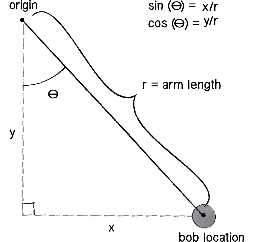
Fig:Position for (x1,y1) co-ordinates.

We can find the value of bob at different location of 'theta1' that is our angular displacement. Thats the reason, we will use our 1st column of result, as it has our result of angular displacement.

From above figure r = L;

x = x1;

y = y1;

and the pendulum is hung at origin (x0,y0) =(0,0).

Here, we will use a for loop for 'i' starting from one to length of our array result storing displacement values. Basically this, will iterate for 500 variables.

The hanging position x0,yo does not change. But for x1 and y1, our displacement value will change at every iteration and so will our x1 and y1 position.

The equations are;

x1=L*sin(result(i,1));

y1=-L*sin(result(i,1));

For every iteration, 'i' will change but column will remain same. This brings about a change in x1 and y1 value during every iteration. Note that the sign before cosine element is negative, because we want our simulation taking place down, not other way round.

Now using plot([x0,x1],[y0,y1]) are pendulum length that is L is plotted and for illustation given thickness 2.5 mm and colour green. As L is constant, the length of string wil not change at any point during simulation

Using the code 'plot(x1,y1,'o','MarkerSize',15,'MarkerEdgeColor','b','MarkerFacecolor','r')' we have actually made our pendulum bob using marker and have set some specification to marker. The position of pendulum will change with string, as a result we have plotted it as x1 and y1

Using the code 'plot([-1,1],[0,0])' we will plot the hanging line and mention Linewidth as 2 mm and colour of line as cyan

For better illustration, I have mentioned the hanging point using marker command ' plot(x0,y0,'s','MarkerSize',7.5,'MarkerEdgeColor','b','MarkerFacecolor','r')' and this point is stationary. We will give other markeer specification as per our convenience.

We will put all this in figure(2)

We have used hold on before making first plot to safeguard its result. We will need to mention hold off command too after plotting movement of string and ball. If it is not mention, we will get the below error;

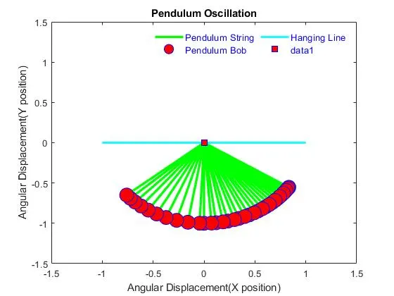
Fig: Plotting without 'hold off' does not removes the last plot of ball and string.

Hence, we will use hold off to remove position of string and ball at prior location

Using xlabel, ylabel and title we have named X-cordinate, Y-co-ordinate and Title of graph, respectively.

Using the below code 'legend('Pendulum String','Pendulum Bob','Hanging Line','FontSize',10,'TextColor','blue','NumColumns',2)', we have named our line and marker corresponding to the plots code written order. The fontsize of the naming is 10 in blue colour. Numcolumns = 2 actually split the naming into 2 columns.

Axis function {axis([-1.5 1.5 -1.5 1.5])} is used show that we can get our actual co-ordinates necessary to plot the figures and ultimately make animation.

The pause function actually pauses the frame for the specified amount of time. 'pause(0.01)' takes a pause of 0.01 sec in every frame and it ultimately reflects in our video.

Here, once all frame is captured, we will make a video out of it using movie function. Movie will take the input as frames stored in A. We will make a variable videofile, where we use function VideoWriter. Here, we store the name of video in 'avi' format in uncompressed version. Then, we actually start video making using open function, where the name of the video that will be created will be 'Pendulum Oscillation'. Then we use writeVideo function to create the video of the name 'Pendulum Oscillation' in uncompressed version with the frames stored in A. Once that is done, we will use close function of videofile.

Result:

The plot of 'Result v/s Time' is ;

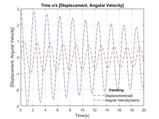
Fig: Plot of Time against Result

Here, blue curve denotes the graph of 'Time against Angular Velocity' and red curve denotes 'Time against Displacement'

The simulation of 'Oscillation of Pendulum is:

Learning Outcome:

• Understood the Second Order Differential Equation of a 'Simple Pendulum' motion
• Learned to use inbuilt function 'ode45'.
• Learned to create ode function.
• Learned to simulate the 'Oscillation of a Pendulum' using ode function

Conclusion:

Created a program in MATLAB by making an 'ode' function for an 'Oscillation of a Simple Pendulum' and simulated its motion. Also, plotted graph of Time against 'Angular Displacement' and 'Time against Angular Velocity'.