Week 3 - Solving second order ODEs

AIM:

Write a program for solving 2nd order differential equation in Matlab

About 2nd ode of Simple Pendulum:

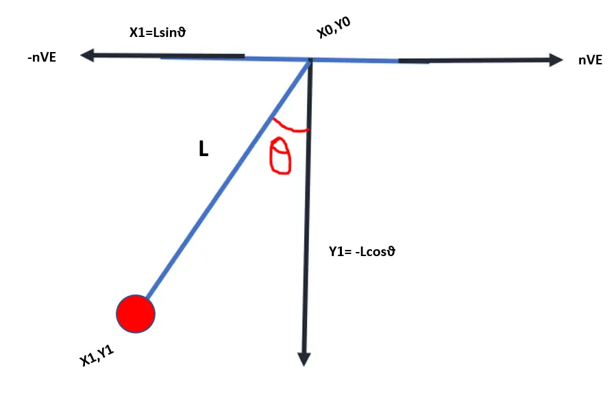
The Equation is

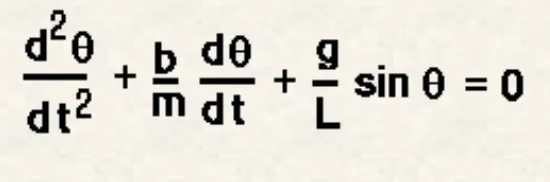.................eq1

In the above equation,

g = gravity in m/s2,

L = length of the pendulum in m,

m = mass of the ball in kg,

b=damping coefficient.

Let us assume that

therefore

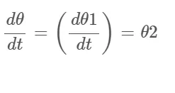............................................eq2

so

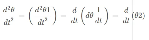.............................eq3

Substituting eq2 in eq1 we get

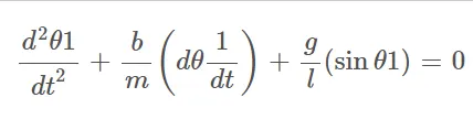
which equals to...

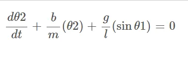
Therefore:

&

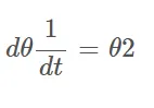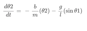
Program for the function creation for ode solver:

So our first function creation is based on the above equation

function [dtheta_dt] = ode_func(t,theta,b,g,l,m)
    
theta1 = theta(1)
theta2 = theta(2)
dtheta1_dt=theta2;
dtheta2_dt = -(b/m)*theta2 - (g/1)*sin(theta1);
dtheta_dt = [dtheta1_dt;dtheta2_dt];
end 

Program for the Ode solver including the animation and graph of Angular Displacement Vs Time

clear all
close all
clc

b=0.05;  %Damping coeffiecient
g=9.81;  %Gravity in m/ss2
l=1;     %length of Pendulum in metre
m=1;     % Mass of pendulum in kg

%Initial condition
%Simulate the motion between 0-20 sec
%angular displacement=0
%angular velocity=3 rad/sec at time t=0
theta_0=[0;3];
%Time Junctions

t_span = linspace(0,20,400);  %time span divided in 400 parts
%ODE fucntion & solver

[t,results]=ode45(@(t,theta) ode_func(t,theta,b,g,l,m),t_span,theta_0);
 
plot(t,results(:,1))
figure(1)

hold on
grid on
plot(t,results(:,2))
ylabel('Angular Displacement & Velocity')
xlabel('time')
legend('Displacement in given angular limits','Angular Velocity')


%origin point hold

figure(2)
hold on
x0=0
y0=0
ct=1

% Pendulum Oscilation Plot

for v=1:length(t) % variable v for constantly changing angular displacements
    x1=l*sin(results(v,1))  %oscilation direction of pendulum in x axis
    y1=-l*cos(results(v,1)) %oscilation direction of pendulum in -ve y axis
    
    plot([x0 x1],[y0 y1],'linewidth',4, 'color','b')  
    hold on
     plot([-0.5 0.5], [0 0], 'linewidth',4,'color','g')
     hold on
     
     %Dipiction of approx end of oscillation
      plot([-1 -0.5],[-0.5 -0.5], 'linewidth',4,'color','r') 
      hold on
       plot([0.5 1],[-0.5 -0.5], 'linewidth',4,'color','r')
       hold on
     
   hold on
   plot(x1,y1,'o','markersize',15,'markerfacecolor','w')
   
   axis([-2 2 -2 2])
   
   grid on
   hold off
   pause(0.0001)
   M(ct)=getframe(gcf);
   ct=ct+1;
end
   %Video File 
   movie(M)
   videofile = VideoWriter('ode_func_main.avi','Uncompressed AVI');
   open(videofile)
   writeVideo(videofile,M)
   close(videofile)
   
    




    

Result Graph of Angular velocity/displacement vs time span (0-20)

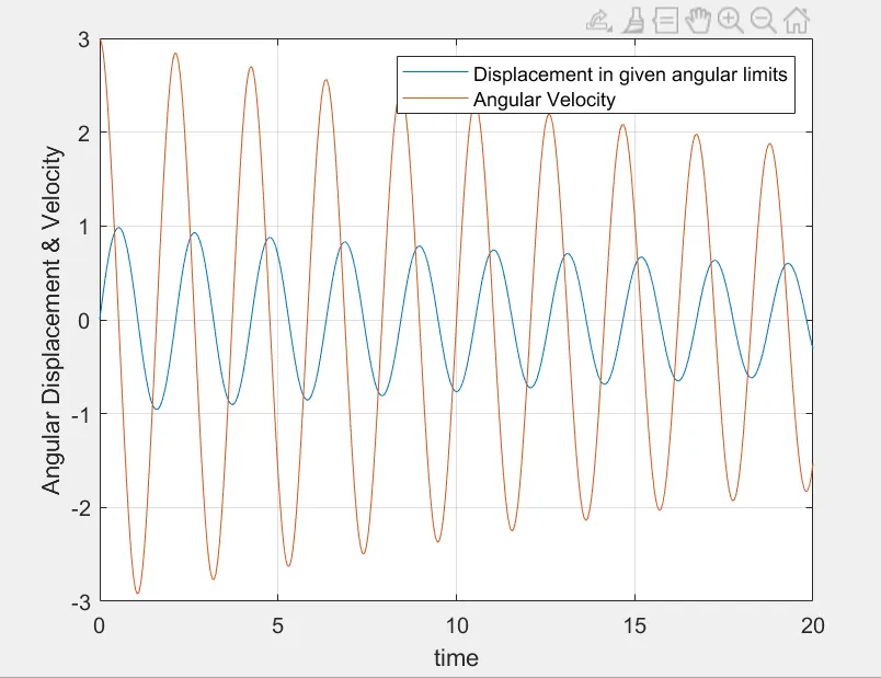
LINK FOR THE ANIMATION VIDEO OF OSCILLATION FOR SIMPLE PENDULUM

https://drive.google.com/file/d/1_mbWtzYY_wf4Es5V0CEjuEj34EdMim-T/view?usp=sharing

CONCLUSION

The creation of a program using ode45 function (for converting 2nd ode into 1st ode) is done and animation for the simple pendulum is completed