Week 3 - Solving second order ODEs

AIM

To write a program that solves the following ODE in MATLAB. This ODE represents the equation of motion of a simple pendulum with damping

and Write a program to simulate the pendulum motion.

PROCEDURE

1. To write a program that solves the following ODE

Simple Pendulum

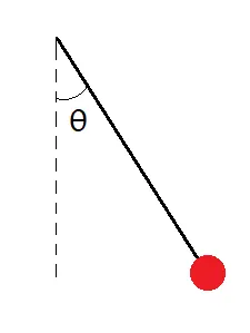
Equation

where,

g = gravity in m/s2, L = length of the pendulum in m, m = mass of the ball in kg, b=damping coefficient.

Values given

L=1 metre, m=1 kg, b=0.05, g=9.81 m/s2.

The above equation is the second order ODE(Ordinary Differential Equation). Solving this equation for θ and the rate at which the θ value is changing with respect to time(velocity).

let us say

θ = θ1

Then dθ/dt = dθ1/dt = θ2 --- (Relation 1)

Here d²θ/dt² = d²θ/dt² = d/dt(dθ1/dt) = d/dt(θ2) --- (Relation 2)

Now θ = θ1 in

d²θ/dt² + b/m dθ/dt + g/L sin θ = 0

So we have

d²θ1/dt² + b/m dθ1/dt + g/L sin θ1 = 0

Here d²θ1/dt² = dθ2/dt ; From equation 1 --> θ2 = dθ1/dt

So, dθ2/dt + b/m θ2 + g/L sin θ1 = 0

In order to solve the second order ODE, we have created two ODEs i.e

dθ1/dt = θ2 and dθ2/dt + b/m θ2 + g/L sin θ1 = 0. Now we have two first order ODEs.

Now let us say

d/dt[θ1 θ2] = [θ2 -b/m θ2 - g/L sin θ] since it contains two quantities we call it as a soution vector. and we take d/dt[θ1 θ2] as θ.

Now, let us start writing the program. Under Editor > Open a new script window > First we start with the basic flow and define the inputs of g = gravity in m/s2, L = length of the pendulum in m, m = mass of the ball in kg, b=damping coefficient.

Next we define the initial conditions. Initially to solve the first order ODE we have to provide the displacement. Here initial displacement of the pendulum is '0' and initial velocity is '3' m/sec.

Now we integrate the ODE system for solution by which we define the value for time. Write t_span (which is nothing but the time array) which goes from '0' to '20' seconds between '500' values.

[Calling the ODE function

To do so, Under Editor > Open a new script window > then in the function we type in ODE45 which is a solver in MATLAB and then we define our ODE as a function of 't' and 'theta'. Then we define our function ODE with t, theta, damping coefficient, gravity, length of the pendulum and mass. In t_span we provide the initial condition, integration and time array. And finally the initial condition corresponding to the starting of the time.

Here we define theta1 and theta2. Then we define the first order ODE dtheta1_dt = theta2. And for the second order ODE dtheta2_dt = -(b/m)*theta2 - (g/1)*sin(theta1). Finally we combine them with an array i.e dtheta_dt = [dtheta1_dt; dtheta2_dt] with two rows. Hence it is a column matrix. And end with the end command.]

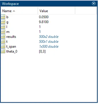
The call function will give the 'time', 'integration time' and the 'results'. We solve two ODEs and it's a column vector we specify it as two columns. Inorder to see that go to workspace > open results and we can see that it shows two columns where the first column refers to the 'displacement' and the second column refers to the 'velocity'. The values start with [0,3] as per our initial displacement and velocity.

Then plot them by plot(t,results(:,1)) and use 'hold on' command then plot (t,results(:,2)). Name ylabel as ('plot') and xlabel as ('time'). Now run the program. The plot graph appears. We can see that there are three curves. The first curve starts from '0' is the displacement and the second curve starts with '3' is the velocity. The plot graph is shown in the below Fig.

SCRIPT WINDOW

clear all
close all
clc


b = 0.05;
g = 9.81;
l = 1;
m = 1;

% Initial condition
theta_0 = [0,3];

% Time points
t_span = linspace(0,20,500);

% Solve ODE
[t, results] = ode45(@(t,theta) ode_func(t, theta, b,g,l,m),t_span, theta_0);

plot(t, results(:,1))
hold on
plot(t, results(:,2))
ylabel('Plot')
xlabel('time')

ODE CALL FUNCTION

function [dtheta_dt] = ode_func(t,theta,b,g,l,m)

theta1 = theta(1)
theta2 = theta(2)
dtheta1_dt = theta2;
dtheta2_dt = -(b/m)*theta2 - (g/1)*sin(theta1);
dtheta_dt = [dtheta1_dt; dtheta2_dt];
end

WORKSPACE

PLOT GRAPH for DISPALCEMENT AND VELOCITY

2. To write a program to simulate the pendulum motion.

ANIMATION PROCESS OF A SIMPLE PEDULUM MOTION

To do so, Under Editor > Open a new script window > First we start with the basic flow and define the inputs of g = gravity in m/s2, L = length of the pendulum in m, m = mass of the ball in kg, b=damping coefficient.

Next we define the initial conditions. Initially to solve the first order ODE we have to provide the displacement. Here initial displacement of the pendulum is '0' and initial velocity is '3' m/sec.

Now we integrate the ODE system for solution by which we define the value for time. Write t_span (which is nothing but the time array) which goes from '0' to '20' seconds between '500' values.

then call the function

[t, results] = ode45(@(t,theta) ode_func(t, theta, b,g,l,m),t_span, theta_0)

And set output = results(:,1)

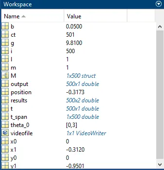
Write in 'for' i = 1:length(output) Here, length(output) refers to the values of 'output'. Each time the value changes, It will execute the set of commands present inside the 'for loop'. and write position = output(i) here, we need to use the loop counter variable 'i' to access the particular value.

'x0' and 'y0' is set as 0 because, it is the starting point of the base. And 'x1' is set as l*sin(position) and 'y1' is set as -l*cos(position)

Feed in a single 'plot' statement as

[x0 x1],[y0 y1],x1,y1,'o','markersize',25,'markerfacecolor','r','markeredgecolor','r' and set the 'linewidth' parameter with a thickness of 3. Then we have to set the 'axis' as [-1.3 1.3 -1.3 1.3] 'the length of the string' And we add the 'pause' command with (0.03). Then write hold off ['hold off' - sets the hold state to off so that new plots added to the axes clear existing plots and reset all axes properties. The next plot added to the axes uses the first color and line style based on the ColorOrder and LineStyleOrder properties of the axes. This option is the default behavior.] Then add the title command to name it as 'Pendulum Motion'. Turn on the Grids. In order to make it as a movie in frames > we use an array called 'M'. i.e M(ct) = getframe(gcf). so by using 'getframe' we get a particular figure window and save it in an array called 'M'. And each time 'for loop' is excecuted we increment it with counter ct = ct + 1. Also add 'ct=1' before 'for loop' command. And end withv'end' command. Now at the end of the 'end' command we write in as movie(M) where MATLAB will generate a movie with all the frames.

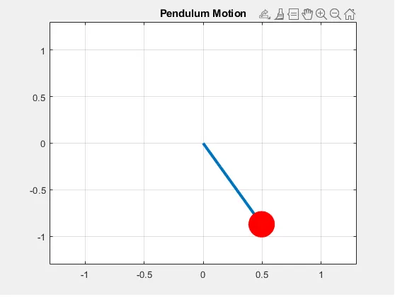
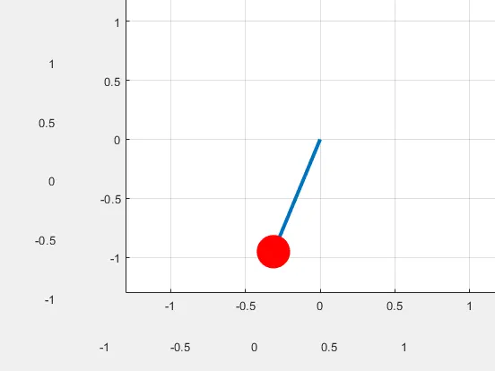
In order to save the frame as a video le in AVI format we write a command as videole = VideoWriter('pendulum_motion.avi','Uncompressed AVI') so we have given the lename along with a format. After this we have to set a 'open' command 'open(videole)'. Then 'writeVideo(videole,M)' we say it to write the video with the frames we have. And finally we set it as 'close(videole)'. So now, When we run the program we can see that a video le has been saved in our current folder. And also the plot graph animation playing as shown in the below Fig.

SCRIPT WINDOW

clear all
close all
clc

b = 0.05;
g = 9.81;
l = 1;
m = 1;

% Initial condition
theta_0 = [0,3];

% Time points
t_span = linspace(0,20,500);

% Solve ODE
[t, results] = ode45(@(t,theta) ode_func(t, theta, b,g,l,m),t_span, theta_0);

output = results(:,1)

ct=1;
for i = 1:length(output)
    position = output(i);
 
 x0 = 0;
 y0 = 0;

 x1 = 1*sin(position);
 y1 = -1*cos(position);

 %Ploting
 
 plot([x0 x1],[y0 y1],x1,y1,'o','markersize',25,'markerfacecolor','r','markeredgecolor','r','linewidth',3)
 axis([-1.3 1.3 -1.3 1.3])
 pause(0.03)
 hold off
 title('Pendulum Motion')
 grid on
 M(ct) = getframe(gcf);
 ct=ct+1;

end
movie(M)
videofile = VideoWriter('pendulum_motion.avi','Uncompressed AVI');
open(videofile)
writeVideo(videofile,M)
close(videofile)

WORKSPACE for PENDULAM MOTION

PLOT GRAPH ANIMATION for PENDULUM MOTION

That is how we create an animation and save it as a movie i.e a video le in AVI format. The created video is embedded at the end of the page.

Animated Video of the PENDULUM MOTION

No errors were found.