Week 3 - Solving second order ODEs

Solving second order ODE's using a simple pendulum :

Main program :

clear all
close all
clc

% inputs
b = 0.05;
g = 9.81;
L = 1;
m = 1;

% initial conditions
theta_0 = [0;3];

% time points
t_span = linspace(0,20,100);

% solving ODE
[t,results] = ode45(@(t,theta) ode_fun(t,theta,b,g,L,m),t_span,theta_0);

% plotting
figure(1)
plot(t,results(:,1))
hold on
plot(t,results(:,2))
xlabel('TIME')
ylabel('DISPLACEMENT')

figure(2)
ct = 1;
for i = 1:length(t_span)
    x_fixed = 0;
    y_fixed = 0;
    x_free = L*sin(results(i,1));
    y_free = -L*cos(results(i,1));
    plot([x_fixed x_free],[y_fixed y_free],[-1 1],[0 0],'linewidth',2)
    hold on
    plot(x_free,y_free,'marker','O','markersize',25,'markerfacecolor','r')
    hold off
    axis([-1.5 1.5 -1.5 0.5])
    title('simple pendulum motion')
    pause(0.2)
    M(ct)=getframe(gcf);
    ct = ct + 1;
end

movie(M)
videofile = VideoWriter('ode_function.avi','uncompressed AVI');
open(videofile)
writeVideo(videofile,M)
close(videofile)

ODE function program to be used in the main program :

function[dtheta_dt] = ode_fun(t,theta,b,g,L,m)
    theta1 = theta(1);
    theta2 = theta(2);
    dtheta1_dt = theta2;
    dtheta2_dt = -(b/m)*theta2 - (g/L)*sin(theta1);
    dtheta_dt = [dtheta1_dt;dtheta2_dt];
end

Objective :

The main objective of this program is to solve ODE from complex equations. Here the motion of the simple pendulum is used as an example. The equation is known as a second-order differential equation,

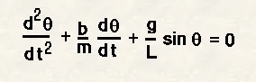
from the above equation, we can break it into two first-order equations. They are as follows, `(d theta_1)/dt = theta_2` and `(d theta_2)/dt`=-`(b/m)*`theta_2`+`(g/L)`*sin`theta_1`.

By solving the above two ODE's we can solve the given second-order equation.

Code explanation :

Since all the input parameters required to substitute in the equation has been given, we can start the programs from the smaller function program that is to be used in the main program.

Here, function command is used to give a name and all the desired inputs in the program. The values of Theta1 and Theta2 are assigned by the values of respective thetas of 1st and 2nd angles. Both the first-order ODE's are described and the final solution is described as dtheta_dt = [dtheta1_dt;dtheta2_dt]. Finally, the end command is used to finish the function program.

The main program is started using as usual clear all close all and clc commands. Then the given input values are written. The initial condition of the pendulum is given using the theta_0=[0;3]; where 0=displacement and 3=angular velocity. The number of points to be plotted is given using the linspace command, wherein this case 100 values are taken in between 0-20 seconds.

To solve the ODE, the ode45 command is used to define the calculations as ODE calculations to the MatLab. Then the ode_fun program is called in the main program.

for plotting the time-displacement graph, the 1st and 2nd results are plotted with respect to the time. x and y labels of the graphs are given.

Then for animating the pendulum motion, we set the initial values of ct = 1 and the coordinates of the fixed end of the pendulum are given( in this case it is 0,0). then the free end is calculated using x_free = Lsin(i,1) where the first angle is along the y-axis, L of sin theta is used. y_free = -Lcos(i,1).

plotting is used to denote the fixed point of the pendulum. ([x_fixed x_free],[y_fixed y_free],[-1 1],[0 0],'linewidth',2) where both the fixed and free coordinated are calculated and the line length of the fixed point is denoted by -1 to 1. And desired linewidth is used.

hold on command is used to repeat the commands and plotting all the points of the pendulum in a same graph. The free end of the pendulum is plotting and marker commands are used to describe the size and color of the pendulum ball. Hold off command is used so that the animated lines would disappear during the course of the next animation. Axis limits of the x and y limits are given through axis command. Title command is used to print the title of the in the animation.

pause of 0.2 is used to delay the animation. And getframe is used to make the movie. video writer command is used to give the name and file format of the files. finally close video file os used to finish the animation video.

Output :

The output of the program is as follows,

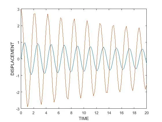
This graph describes the displacement of the pendulum with respect to the time.

https://drive.google.com/file/d/1kU6p69U_0bm2EJztAXEG2C2KsTaNTv6D/view?usp=sharing

Errors faced during programming :

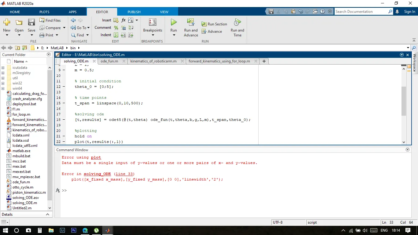
This error is caused because I failed to mention the length of the fixed-line length.

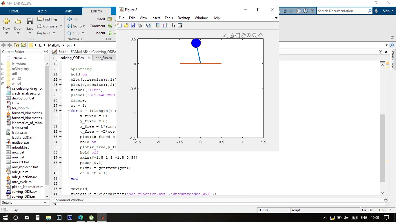
This error is caused because while calculating the Y_free point, I used cos(results(i,2)) instead of results(i,1).

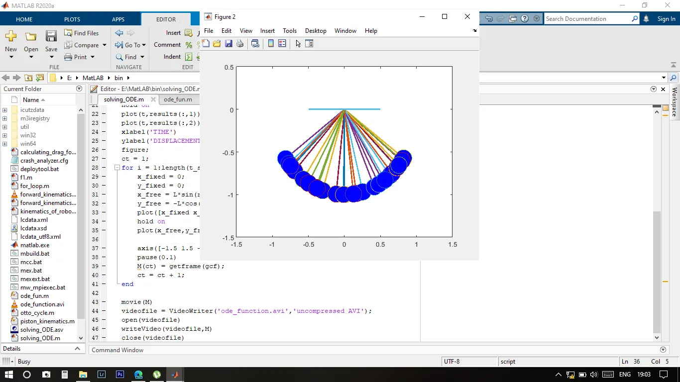
Hold off command is not used at first, causing this error. After connecting with the mentor, hold off is used and the error is rectified.