Week 3 - Solving second order ODEs

AIM:- To write a program that solves the ODE that represents the equation of motion of a simple pendulum with damping and to create a simulation of simple pendulum using image magic.

formula :`(d^2theta)/(dt^2) +b/m*(d theta)/(dt) + g/l*sin theta = 0`

where b=damping co efficient

g= acceleration due to gravity(9.81 m/s^2)

l=length of the pendulum string

m= mass of the body(bob) attached to the string

now if we consider`theta =theta_1`(displacement)

`(d theta)/(dt) =(d theta_1)/(dt)=theta_2`[where `theta_2` represents the velocity of the bob]

and `(d^2theta)/dt^2=(d^2theta_1)/dt^2=(d)/(dt) ((d theta_1)/(dt))=(d theta_2)/(dt)`

on substituting to the original equation we get,

`(d theta_2)/dt=-b/mtheta_2 -(g/l)sin(theta_1)`

and hence we got two first order ODE from the basic second order differential equation.

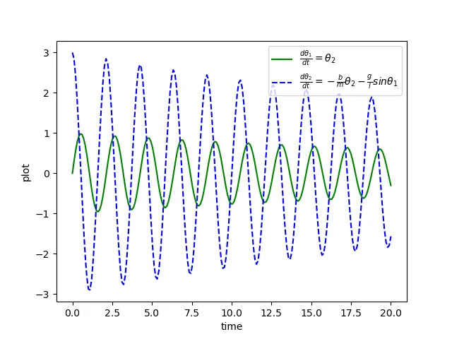
by using this two first order ODE we can create a program to solve the given ODE and create a plot with the obtained data.

later we can create a simulation of simple pendulum by cosidering one end of string fixed hence its co ordinates being at origin and coordinates of other end of the string is (lsin`theta` ,-l`cos theta`).

the program is as follows,

import numpy as np
from scipy.integrate import odeint
import matplotlib.pyplot as plt
import math
def model(theta,t,b,g,l,m):
	theta1=theta[0]
	theta2=theta[1]
	dtheta1_dt =theta2
	dtheta2_dt= -(b/m)*theta2 -(g/l)*math.sin(theta1)
	dtheta_dt =[dtheta1_dt, dtheta2_dt]
	return dtheta_dt

#input variables	
b=0.05
g=9.81
l=1
m=1

# initial condition	
theta_0 =[0,3]
#time points
t=np.linspace(0,20,200)

#solve ode
theta= odeint(model,theta_0,t,args=(b,g,l,m))

plt.plot(t,theta[:,0],'g-',label=r'$\frac{d\theta_1}{dt}=\theta_2$')
plt.plot(t,theta[:,1],'b--',label=r'$\frac{d\theta_2}{dt}=-\frac{b}{m}\theta_2-\frac{g}{l}sin\theta_1$')
plt.xlabel('time')
plt.ylabel('plot')
plt.legend(loc='best')
plt.show()

#creating simulation of simple pendulum

x0=0
y0=0
theta =theta[:,0]
ct=1
for t in theta:
	x1=-l*(math.sin(t))
	y1=-l*(math.cos(t))
	stallone='test%05d.png' % ct
	ct=ct+1
	plt.figure()
	#plot of the support
	plt.plot([-1.5,1.5],[0,0],linewidth=5)
	#plot of the string
	plt.plot([x0,x1],[y0,y1],linewidth=3)
	#plot of bob
	plt.plot(x1,y1,'o',markersize=20)
	plt.xlim([-1.5,1.5])
	plt.ylim([-1.5,1.5])
	plt.savefig(stallone)

output:-

https://www.youtube.com/watch?v=jDOKODMI8Nk&feature=youtu.be