Week 3 - Solving second order ODEs

SECOND ORDER ODEs

In Engineering, ODEs(ordinary differential equations) describe various transient systems.

The motion of a simple pendulum with damping can be understood with the help of the following ODE :

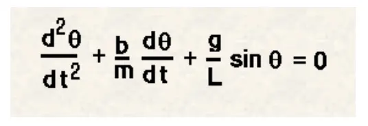
where,

g = gravity in m/s2

L = length of the pendulum in m

m = mass of the ball in kg

b=damping coefficient.

OBJECTIVE : Write a Python code to solve the given ODE and to animate the motion of a pendulum.

PROBLEM STATEMENT:

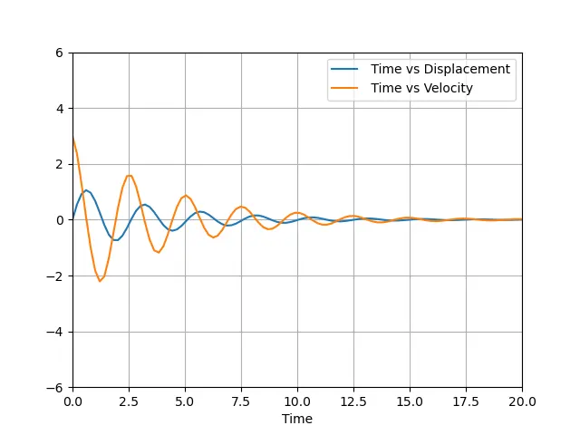
Solve the ODE using ODEINT module and plot the output(ang disp and ang vel) vs Time.

Also, Simulate the motion between 0-20 sec, for angular displacement=0, angular velocity=3 rad/sec at time t=0.

SOLUTION PROCEDURE:

Preliminary Equations:

Firstly we transform the 2nd Order Order ODE into two 1st order ODEs .

PYTHON CODE :

from scipy.integrate import odeint
import math
import matplotlib.pyplot as plt 
import numpy as np 



# Converting the second order differential equation in two first order diff eqns( also function form)
def function(theta,t,b,g,l,m):

	theta1 = theta[0]
	theta2 = theta[1]
	dtheta1_dt = theta2
	dtheta2_dt = -(b/m)*theta2 - (g/l)*math.sin(theta1)
	dtheta_dt = [dtheta1_dt, dtheta2_dt]
	return dtheta_dt



# INPUTS
b = 0.05	#Damping coefficient
g = 9.81	#Accn due to grav
l = 1.5		#Length
m = 0.1		#Mass

#Initial Conditions

theta_0 = [0,3]


#Time Array
t = np.linspace(0,20,100)

#Solving THe Differential Equation using ODEINT solver
theta = odeint(function,theta_0,t,args = (b,g,l,m))


a = theta[:,0] 


#PLOTTING TIME v/s DISP AND VELOCITY

plt.figure()
plt.plot(t,theta[:,0],label=' Time vs Displacement')
plt.plot(t,theta[:,1],label= ' Time vs Velocity')
plt.legend()
plt.xlabel('Time')
plt.xlim([0,20])
plt.ylim([-6,6])
plt.grid()
plt.show()


x0 = 0
y0 = 0

ct = 1

for A in a:

	x1 =  l* math.sin(A) 
	y1 = -l* math.cos(A)

	
	filename = 'ODE%05d.png' %ct
	ct = ct+1

	plt.figure()
	plt.plot([-2,2],[0,0],linewidth = 2, color = 'blue')
	plt.plot([x0,x1],[y0,y1],linewidth = 3)
	plt.plot(x1,y1,marker = 'o',color = 'red', markersize = 13)
	plt.xlim([-3,3])
	plt.ylim([-3,3])
	plt.savefig(filename)

RESULTS:

(A)Time vs ANG DISP. & ANG. VEL.

(B)SIMULATION OF PENDULUM (VIDEO):

Animation made using ImageMagick.

CONCLUSION: Due to the damping provided to the pendulum , the oscillations are slowly dying and eventually stop. So do the graphs for angular disp and angular velocity.