Week 3 - Solving second order ODEs
OBJECTIVE:
To write a Matlab program that solves the ODE of a Simple pendulum.
THEORY:
Pendulums have many applications and were utilized often before the digital age. They are used in clocks and metronomes due to the regularity of their period, in wrecking balls and playground swings, due to their simple way of building up and keeping energy. They are even found in various scientific instruments, from seismographs to early torpedo guidance systems, due to their sensitivity to disturbance.
The simple pendulum consists of a point mass ('m') hanging on a string of length of ('l') from some support. The vertical line passing through the fixed support is the mean position of a simple pendulum. The vertical distance between the point of suspension and the centre of mass of the suspended body(when it is in mean position) is called the length of the simple pendulum denoted by l.
From Newton's second law of motion ,
F=ma
where,
F--Force(N)
m--mass(kg)
a--acceleration(m/s^2)
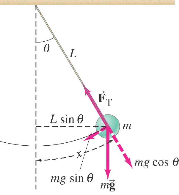
From the fig, it is evident that there are two forces acting on the point mass. The first is gravity. This point downward and has a magnitude of mg, where g is the standard symbol for the acceleration due to gravity. The other force is the tension in the string. The net force is found to be -mgsin`theta`.
Equating Newton's second law and above net force we get,
m`x¨ = −mg sin θ.`
Next, we need to relate x and θ. x is the distance travelled, which is the length of the arc traced out by the point mass. The arclength is related to the angle, provided the angle is measure in radians. Namely, x = rθ for r = L. Thus, we can write:
`mL ¨θ = −mg sin θ`
Cancelling the masses, this then gives us the nonlinear pendulum equation,
L ¨θ + g sin θ = 0.
If we Consider the damping, then the equation becomes:
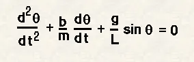 --------------------------------------1
b=damping coefficient
m = mass at the swinging end of the pendulum (kilograms)
g = acceleration due to gravity (meter/second^2)
L = length from the swivel point to the centre of mass (meters)
θ = angle between the string position to the string position at rest (radians)
t = time (seconds)
If we solve this particular differential equation basically we are solving for theta and also the rate at which theta value changes with respect to time.
To solve the Higher-order differential equations ,we need to breakdown it into two first-order differential equations.
`theta=theta1`--------------2
`(d theta)/dt=(d theta1)/ dt=theta2`--------3
`(d ^2 theta)/dt^2=(d^2 theta1)/dt^2=d/dt((d theta1)/dt)=d/dt(theta2)`------4
Equation 1 becomes,
`(d^2 theta 1)/dt^2+b/m (d theta1)/dt+g/lsin theta1=0`--------------(using 2)
`(d theta 2)/dt+b/m theta 2+g/lsin theta 1=0`--------------------------(using 3 and 4)
`(d theta 2)/dt= -b/m theta2 -g/lsin theta1`
`d/dt(theta)=[theta 2 ; -b/m theta2 -g/lsin theta1]`
Thus, we breakdown the second-order differential equation into two first-order differential equations.
MATLAB PROGRAM:
clear all
close all
clc

b=0.05;
g=9.81;
l=1;
m=1;

%initial condition

theta_0=[0;3];

%Time inputs

t_span=linspace(0,20,500);

%Solve ODE

[t,results]=ode45(@(t,theta) ode_func(t,theta,b,g,l,m),t_span,theta_0);

ct=1;

for i=1:length(results(:,1))

    x0=0;
    y0=0;

    x1=l*sin(results(i,1));
    y1=-l*cos(results(i,1));


    plot([-1,1],[0,0],'linewidth',3,'color','r');
    hold on

    plot([x0 x1],[y0 y1],'linewidth',2,'color','g')

    hold on
    plot(x1,y1,'o','markers',20,'markerfacecolor','b');
    grid on
    title('Simulation of a Damped Pendulum')
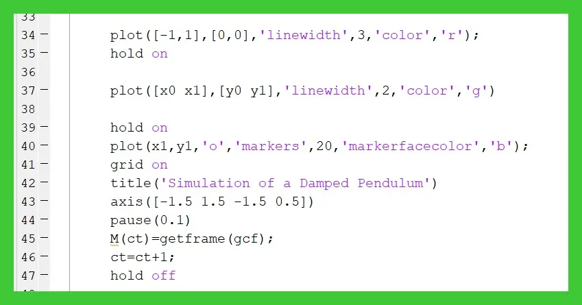
    axis([-1.5 1.5 -1.5 0.5])
    pause(0.1)
    M(ct)=getframe(gcf);
    ct=ct+1;
    hold off

end

movie(M)
videofile=VideoWriter('simple_pendulum.avi','Uncompressed Avi');
open(videofile)
writeVideo(videofile,M)
close(videofile)

figure(2)
plot(t,results(:,1))
hold on
plot(t,results(:,2))
grid on
xlabel('Time (s)')
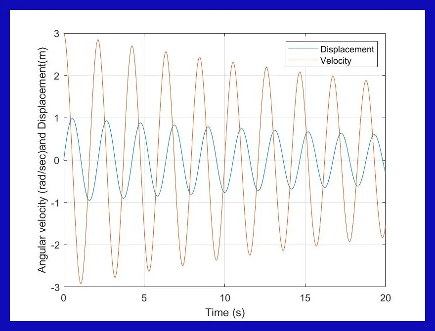
ylabel('Angular velocity (rad/sec)and Displacement(m)')
legend('Displacement','Velocity')
STEPWISE EXPLANATION:
- The program starts with the command clear all, close all, and clc in order to clear all the data stored in the workspace, plot, and command window.
- The inputs are defined which includes damping coefficient(b), acceleration due to gravity(g), length of the string(l), the mass of the bob(m).
- Then, the initial condition for displacement and velocity is defined and it stored in theta_0.
- Then, the timepoint up to which the integration needs to be done is defined.
- Then using the ode function the results are obtained.
- ode45 defines the function.ode_func defines how the ode function is defined.t_span defines the time span how far the integration needs to be done. At last,theta_0 defines the initial condition of displacement and velocity.
- The ode_func is defined in a separate program and it is called in the main program.
- The counter value ct is defined initially as 1.
- Then for loop is defined with i equal to 1 to the length of the column1 matrix in results(ie displacement).
- Initial coordinates for x and y value is set as zero.
- To calculate x1 and y1 the formula is defined,
- x1=l*sin(results(i,1))
- y1=-l*cos(results(i,1))
- Then the top line of the pendulum is defined on which the string is attached.
- Then the string is defined by plotting x0, x1,y0and y1 values.
- Then the bob is defined by using the markers command.
- Then the title and axis are defined.
- Then the frame is stored in the M array in order to create a movie.
- Then the counter is incremented and the program repeats.
- Then to make an animation movie command is defined. The stored images are now assigned to the movie command.
- Then video file is created with the filename and the format is defined for the video file.
- Then using the open command the video file is opened and using the write video command the video is written in the file which is mentioned above.
- Then using the close command the file is closed.
- Figure 2 is defined by plotting time(s) vs displacement (m) and angular velocity(rad/s)
Sub-Program:
function[dtheta_dt]=ode_func(t,theta,b,g,l,m)

theta1=theta(1)
theta2=theta(2)

dtheta1_dt=theta2;
dtheta2_dt=-(b/m)*theta2-(g/l)*sin(theta1);
dtheta_dt=[theta(2);dtheta2_dt];


end
- The ode function is defined with inputs t, theta,b,g,l and m.
- Based on the above splitting of the second-order differential equation into two first-order differential equation, it is defined inside the program.
ERRORS:
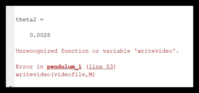
- The command write video is not defined properly because in the write video command the V letter must be in upper case. It's a predefined function so we have to type it in the same way as defined.
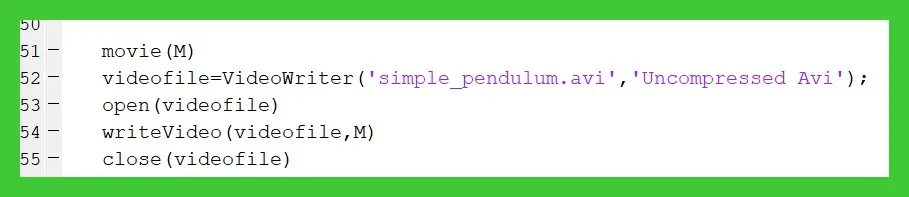
2)Error in Animation:
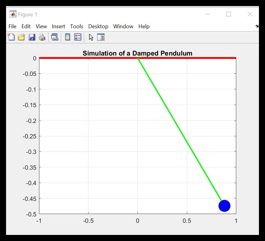
- Due to the axis is not defined in the program the y-axis is deflected more according to the change in the displacement values. Even though this error is not shown in the command window, the animation looks inappropriate due to the y-axis is not fixed. This error can be rectified by fixing the axis properly.
RESULTS:
- Thus a program is written for the simulation of a simple pendulum according to the given input values.
- The video file is generated for the simulation.
PLOT:
Youtube video link for animation:
LEARNING OUTCOMES:
- Understand the basis of a simple pendulum and its equations more clearly.
- Understand how to split the Higher-order differential equation into simple first-order differential equations.
- Understand how to simulate an ODE.