Finding maximum of a function using Genetic Algorithm in Matlab.
Aim: To determine the maximum of a function using genetic algorithm.
Introduction:
Genetic Algorithm is an optimisation technique in which we use an iterative process to determine the best suitable value for the variables of function to minimize it.It is used for solving both constrained and unconstrained optimization problems based on a natural selection process that mimics biological evolution.
Genetic Algorithm Terminology
The assigned data points undergoes following steps:
- Selection: The parents are selected in this process which will form the initial population. The selection process takes place in such a way that it selects the data set which has higher fitness value.
- Crossover: In this step, a pair or set of parents or data points are selected to form a new offspring which will be then used as sample data set.
- Mutation: This step is carried out to preserve the genetic diversity of the upcoming population.
# Fitness Function:
There is a seperate .m file we generate in which we define the fitness function as anonymous function. This Function takes the data points as inputs and helps to converge the genetic algorithm towards maximum function value.
Note: In this example it is possible to conclude the maximum or minimum value, but in a complicated data set where there are plenty of local minima and maxima, it is quite difficult to differentiate. The problem even gets complicated when the no. of input variable increases. Hence genetic algorithm converges towards the optimum function value where the fitness function defines it as equal to or close to the maximum or minimum.
If maximum value of a function needed to be determined, then we insert a minus sign while defining the fitness function. Also we insert minus sign while plotting the graph so as it invert the graphical results.
Genetic Algorithm terminates when-
-When there has been no improvement in the population.
-When we reach the predetermined number of generation.
-When the objective function has reached the predefined value.
# the function file for this project is saved as a separate .m file and is given as follows:
function [F] = stalagmite(input);

         a = input(1)
         b = input(2)

         f1_x = (sin(5.1*pi*a + 0.5)).^6;
         f1_y = (sin(5.1*pi*b + 0.5)).^6;
         f2_x = exp(-4*log(2)*((a-0.0667)^2/0.64));
         f2_y = exp(-4*log(2)*((b-0.0667)^2/0.64));


         F = -(f1_x*f1_y*f2_x*f2_y);
end
Case study 1:
In this study we will create a search pool by "linspace" command. A 2D matrix is created with "meshgrid" command by using the x and y values. Then we create input vectors inside a "for loop". So the input_vector(1) and input_vector(2) are arrays for the plot. Then we assign these input vectors to the stalagmite function which we create as an anonymous function in a separate .m file.
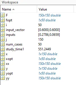
Now to call the algorithm, we assign the stalagmite function to "ga" inside a "for loop" for a number of iterations. Here in code we take it as num_cases = 50. tic and toc command is used to record the time taken to complete the algorithm.
the code for unbounded constraints case is as follows:
clc
close all
clear all

% defining search space
x = linspace(0,0.6,150);
y = linspace(0,0.6,150);
num_cases = 50
% creating a 2dimensional mesh
[xx,yy] = meshgrid(x,y);

% evaluating the stalagmite function

% to create the plot
for i = 1:length(xx)
    for j = 1:length(yy)
        input_vector(1)=xx(i,j);
        input_vector(2)=yy(i,j);
        F(i,j) = stalagmite(input_vector);
    end
end

tic
% to generate the algorithm
% study 1- statistical behaviour
for i = 1:num_cases
    [inputs,fopt(i)] = ga(@stalagmite,2);
    xopt(i) = inputs(1);
    yopt(i) = inputs(2);

end

study_time1 = toc

figure(1)
subplot(2,1,1)
hold on
surfc(xx,yy,-F)
shading interp
plot3(xopt,yopt,-fopt,'marker','o','markersize',5,'markerfacecolor','r')
title('unbounded inputs')
subplot(2,1,2)
plot(-fopt)
xlabel('iterations')
ylabel('function maximum')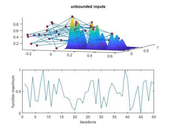
Case study 2
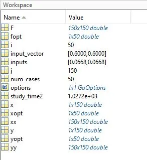
In this case we introduce "optimoptions" and assign it to "ga" solver to specify the population size of the inputs. Also we bound the contraints of the algorithm. We provide the upper and lower bounds so the algorithm can coverge towards the maximum of the function.
the syntax for "ga" is given as -
The code with bounded constraints is as follows:
clc
close all
clear all

% defining search space
x = linspace(0,0.6,150);
y = linspace(0,0.6,150);
num_cases = 50
% creating a 2dimensional mesh
[xx,yy] = meshgrid(x,y);

% evaluating the stalagmite function

% to create the plot
for i = 1:length(xx)
    for j = 1:length(yy)
        input_vector(1)=xx(i,j);
        input_vector(2)=yy(i,j);
        F(i,j) = stalagmite(input_vector);
    end
end

options = optimoptions('ga');
options = optimoptions(options,'populationsize',170);

tic
% to generate the algorithm
% study 1- statistical behaviour
for i = 1:num_cases

    [inputs,fopt(i)] = ga(@stalagmite,2,[],[],[],[],[0:0],[1:1],[],[],options);

    xopt(i) = inputs(1);
    yopt(i) = inputs(2);

end

study_time2 = toc

figure(1)
subplot(2,1,1)
hold on
surfc(xx,yy,-F)
shading interp
plot3(xopt,yopt,-fopt,'marker','o','markersize',5,'markerfacecolor','r')
title('bounded inputs')
subplot(2,1,2)
plot(-fopt)
xlabel('iterations')
ylabel('function maximum')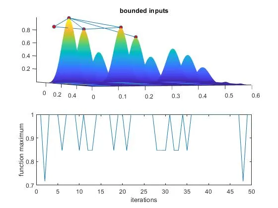
Case study 3
In this case we experiment with the population size and number of iterations to get a converged result.
Keeping the upper and lower bounds as before.
clc
clear all
close all

%study 3 with increased population size and applying constraints
x = linspace(0,0.6,150);
y = linspace(0,0.6,150);
[xx,yy] = meshgrid(x,y);
for i=1:length(xx)
   for j=1:length(yy)

       input(1) = xx(i,j);
       input(2) = yy(i,j);
       f(i,j) = stalagmite(input);
       2
   end
end

tic
options = optimoptions('ga');
options = optimoptions(options,'populationsize',400);
num_cases = 400;

for i=1:num_cases
       [inputs,fopt(i)] = ga(@stalagmite,2,[],[],[],[],[0:0],[0.1:0.1],[],[],options);
       xopt(i) = inputs(1);
       yopt(i) = inputs(2);

end

study_time3 = toc

figure(314)
subplot(2,1,1)
hold on
surfc(xx,yy,-f)

shading interp
plot3(xopt,yopt,-fopt,'marker','o','markersize',5,'markerfacecolor','r')
title('bounded inputs with increased population size')
subplot(2,1,2)
plot(-fopt)
xlabel('iterations')
ylabel('function maximum')
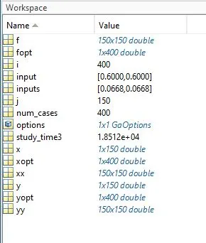
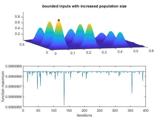
Hence the genetic algorithm is converged to a maximum value of function at x = 0.0668326, y = 0.0668326, z = 1.