Week 3 - Solving second order ODEs

objective:-

to write a program that solves the following ODE. This ODE represents the equation of motion of a simple pendulum with damping

In the above equation,

g = gravity in m/s2,

L = length of the pendulum in m,

m = mass of the ball in kg,

b=damping coefficient.

program:-

import numpy as np
from scipy.integrate import odeint
import matplotlib.pyplot as plt
import math

#function that returns d2/dt
def model(theta,t,b,g,l,m):

	theta1 = theta[0]
	theta2 = theta[1]
	dtheta1_dt = theta2
	dtheta2_dt = -(b-m)*theta2 - (g/1)*math.sin(theta1)
	dtheta_dt = [dtheta1_dt,dtheta2_dt]
	return dtheta_dt

b=0.4	
g=9.81
l=1
m=0.1

#intial condition
theta_θ = [0,5]

 # time point
t = np.linspace(0,20,200)

#solve ODE
theta = odeint(model,theta_θ,t,args = (b,g,l,m))

#plot result
plt.plot(t,theta[:,0],'b-',label=r'$\frac{d\theta_1}{dt}=\theta2$')
plt.plot(t,theta[:,1],'r--',label=r'$\frac{d\theta2}{dt}=-\frac{b}{m}\theta_2-\frac{g}{l}sin\theta_1$')
plt.ylabel('plot')
plt.xlabel('time')
plt.legend(loc='best')

#Polar Co-ordinate To Cartesian Co-ordinate
	y1 = -1*cos(y(0,3));
	x1 = 1*sin(y(0,3));

#Video for Pendulum motion
for i in 90:
	figure(2)
plot([0x1(i)],[0,y1(i)],'linewidth',3,'color','r');
#hold on
plot(x1(i),y1(i),'marker','o','linewidth',10,'markerfacecolor','g');
plot([-1.2,1.2],[0,0],'linewidth',3,'color','b');
axis([-1.2,1.2 -1.2,1.2]);
title(['Time: ', num2str(t_span(i))]);
M(i)is getframe(gcf);
close(2)
end

movie(M)
videofile = VideoWriter('singlependulum.avi','Uncompressed AVI');
open(videofile);
writeVideo(videofile,M)
close(videofile)
#The Function is given as:

#function in ydot = ode_second_order_pendulum(y,b,m,l,g)
#ydot = [y(2);-(b/m)*y(2)-(g/l)*sin(y(1))];
#end

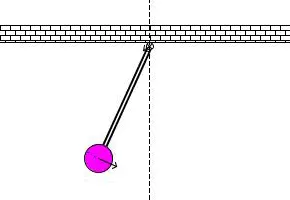
When you do this you will get the position of the pendulum as a function of time. Use this information to animate the motion of the pendulum, as shown in the below figure.