Week 3 - Solving second order ODEs
AIM: TO SIMULATE THE TRANSIENT BEHAVIOR OF A SIMPLE PENDULUM AND TO CREATE AN ANIMATION OF ITS MOTION.
OBJECTIVE :
- To write a program in Python that solves the second-order ODE corresponding to the motion of a simple pendulum and to plot its angular displacement and angular velocity wrt time.
- To create the animation of the motion of pendulum by simulating the motion between 0-20 sec, for angular displacement=0, angular velocity=3 rad/sec at time t=0.
THEORY: A simple pendulum is defined to have an object that has a small mass, also known as the pendulum bob, which is suspended from a light wire or string, such as shown in Figure.
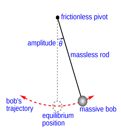
When the bob of the pendulum is displaced from it's mean position to either extreme position and is released, the pendulum will swing back and forth with periodic motion until the motion damps. By applying Newton's second law for rotational systems, the equation of motion for the pendulum may be obtained as.
Procedure:
The 2nd order ODE for a simple pendulum with damping is given below.
d2θ/dt2 + (b/m)dθ/dt + (g/L)sinθ = 0.....(1)
The above ODE is of order 2.To solve it we convert it into two simultaneous ODE of order 1.
Let θ=θ1
and dθ1/dt=θ2...........(2)
Therefore the equation (1) becomes,
dθ2/dt + (b/m)dθ1/dt + (g/L)sinθ1 = 0
⇒dθ2/dt = −(b/m)dθ1/dt − (g/L)sinθ1.........(3)
Here, θ1 is the angular displacement and θ2 is the angular velocity of the pendulum.
- Libraries used:
The following libraries are imported to execute the program.
- matplotlib
Matplotlib is one of the most popular Python packages used for data visualization.
It is a cross-platform library for making 2D plots from data in arrays.
Here in the program,it is used to plot the motion of pendulum with respect to time.
- math
In python a number of mathematical operations can be performed with ease by importing a module named “math” which defines various functions which makes our tasks easier.
Here,math module is used for performing certain trigonometric operations.
- numpy
NumPy is a general-purpose array-processing package. It provides a high-performance multidimensional array object, and tools for working with the arrays.
Here,numpy is used with linspace that returns evenly spaced values within a given interval of time of oscillation of pendulum.(i.e. number of elements are returned).
- scipy
SciPy is a python library that is useful in solving many mathematical equations and algorithms.
The scipy.integrate sub-package provides several integration techniques including solving an ordinary differential equation integrator.
The 'odeint' is a function in the scipy module which integrates the differential equation upto a time step and after getting that solution it keeps on integrating it.
- Variable initialization and declaration:
The following variables are initialized as inputs,
L=1 metre
m=1 kg
b=0.05
g=9.81 m/s2
- Initial conditions:
At t = 0 , angular displacement for the pendulum is 0 and angular velocity is 3 rad per second.These conditions are stored in an array.
- Time points:
A time array of 20 sec with 300 intervals is created upon which the ODE will be solved. It is created using numpy module.
- Defining a new function:
A new function is created with the name simple pendulum.
The inputs of this function are theta (empty array which stores solved answers), t (time array),b (damping coefficient),g (gravitational acceleration), l (length of string) and m (mass of pendulum).
'theta1' is the angular displacement and 'theta2' is the angular velocity.
This function returns an array which has 2 columns and numerous rows.
The 1st column is angular displacement and the second column is angular velocity.
- Solving the ODE:
For 'odeint' command to work properly we pass the differential simple pendulum function, initial conditions, time span and the arguments.
The solved answers are stored in an array of 2 columns 'theta'.
Output:
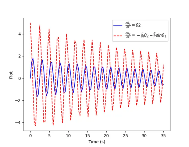
A plot is created between angular displacement versus time and angular velocity vs time
In this plot, blue curve indicates the angular displacement and red dotted curve indicates the angular velocity of the pendulum motion.
As the damping effects are present in the system with a damping coefficient of 3,the amplitude of motion of the pendulum tends to decrease with respect to time.
8.Animation:
Two empty arrays are created to add the values of angular displacements and angular velocities solved in the problem using 'append' command.
The positions of pendulum at fixed end and free end are defined using coordinates.
The position of bob is also defined at the free end of string.
The plots are defined inside a 'for' loop to create an image then and there while the 'for' loop runs for each time with a saved name in sequence.
The created images are then stitched together and converted to animation.
python PROGRAM
"""
TO SIMULATE THE TRANSIENT BEHAVIOR OF A SIMPLE PENDULUM AND TO CREATE AN ANIMATION OF ITS MOTION.
By durga prasad
"""

import matplotlib.pyplot as plt
import math
import numpy as np
from scipy.integrate import odeint

# inputs
m = 1            # (mass of ball in kg)
b = 0.05         # (damping coefficient)
g = 9.81         # (acceleration due to gravity in m/s^2)
L = 1            # (length of string in metres)


def simple_pendulum(theta, t):

    theta1 = theta[0]
    theta2 = theta[1]
    dtheta1_dt = theta2
    dtheta2_dt = - (b / m) * theta2 - (g / L) * math.sin(theta1)
    dtheta_dt = [dtheta1_dt, dtheta2_dt]

    return dtheta_dt


# initial conditions
theta_0 = [0, 5]            # (first element represents the angular displacement in radians and second element represents the angular velocity in rad/sec)

# time points
t = np.linspace(0, 35, 100)

# solving ode
theta_results = odeint(simple_pendulum, theta_0, t)
Angular_Displacement = []
Angular_Velocity = []

# Printing of value angular displacement and angular velocity from the result array using the for loop
for i in range(0, len(theta_results)):

    # Angular Displacement
    angular_displacement = theta_results[i, 0]
    Angular_Displacement.append(angular_displacement)

    # Angular Velocity
    angular_velocity = theta_results[i, 1]
    Angular_Velocity.append(angular_velocity)

#creating animation

ct = 0              #(counter variable)

for j in range(0, len(t)):

    THETA = Angular_Displacement[j]

    OMEGA = Angular_Velocity[j]

    # Defining the coordinates of fixed end of string of the pendulum
    X0 = 0
    Y0 = 0

    # Defining the coordinates of free end of string of the pendulum
    X1 = L*(np.sin(THETA))
    Y1 = -L*(np.cos(THETA))

    #counter variable to store plotted images in different names.

    ct = ct + 1
    filename = str(ct) + '.png'

    #animation  plots
    print(filename)
    plt.plot([-1, 1], [0, 0], color = 'black', linewidth = 10)
    plt.plot([X0, X1], [Y0, Y1], color = 'red', linewidth = 4)
    plt.plot(X1, Y1, marker = 'o', markerfacecolor = 'blue', markersize = 30)
    plt.xlim(-2, 2)
    plt.ylim(-1.5, 0.2)
    plt.savefig(filename)
    plt.close()

#plotting
plt.plot(t, theta_results[:, 0], 'b-',label = r'$\frac{d\theta_1}{dt} = \theta2$')
plt.plot(t, theta_results[:, 1], 'r--',label = r'$\frac{d\theta_2}{dt} = -\frac{b}{m}\theta_2-\frac{g}{L}sin\theta_1$')
plt.xlabel('Time (s)')
plt.ylabel('Plot')
plt.legend(loc = 'best')
plt.show()
shared in google _drive link
"""
TO SIMULATE THE TRANSIENT BEHAVIOR OF A SIMPLE PENDULUM AND TO CREATE AN ANIMATION OF ITS MOTION.
By durga prasad
"""
import matplotlib.pyplot as plt
import math
import numpy as np
from scipy.integrate import odeint
# inputs
m = 1 # (mass of ball in kg)
b = 0.05 # (damping coefficient)
g = 9.81 # (acceleration due to gravity in m/s^2)
L = 1 # (length of string in metres)
def simple_pendulum(theta, t):
theta1 = theta[0]
theta2 = theta[1]
dtheta1_dt = theta2
dtheta2_dt = - (b / m) * theta2 - (g / L) * math.sin(theta1)
dtheta_dt = [dtheta1_dt, dtheta2_dt]
return dtheta_dt
# initial conditions
theta_0 = [0, 5] # (first element represents the angular displacement in radians and second element represents the angular velocity in rad/sec)
# time points
t = np.linspace(0, 35, 100)
# solving ode
theta_results = odeint(simple_pendulum, theta_0, t)
Angular_Displacement = []
Angular_Velocity = []
# Printing of value angular displacement and angular velocity from the result array using the for loop
for i in range(0, len(theta_results)):
# Angular Displacement
angular_displacement = theta_results[i, 0]
Angular_Displacement.append(angular_displacement)
# Angular Velocity
angular_velocity = theta_results[i, 1]
Angular_Velocity.append(angular_velocity)
#creating animation
ct = 0 #(counter variable)
for j in range(0, len(t)):
THETA = Angular_Displacement[j]
OMEGA = Angular_Velocity[j]
# Defining the coordinates of fixed end of string of the pendulum
X0 = 0
Y0 = 0
# Defining the coordinates of free end of string of the pendulum
X1 = L*(np.sin(THETA))
Y1 = -L*(np.cos(THETA))
#counter variable to store plotted images in different names.
ct = ct + 1
filename = str(ct) + '.png'
#animation plots
print(filename)
plt.plot([-1, 1], [0, 0], color = 'black', linewidth = 10)
plt.plot([X0, X1], [Y0, Y1], color = 'red', linewidth = 4)
plt.plot(X1, Y1, marker = 'o', markerfacecolor = 'blue', markersize = 30)
plt.xlim(-2, 2)
plt.ylim(-1.5, 0.2)
plt.savefig(filename)
plt.close()
#plotting
plt.plot(t, theta_results[:, 0], 'b-',label = r'$\frac{d\theta_1}{dt} = \theta2$')
plt.plot(t, theta_results[:, 1], 'r--',label = r'$\frac{d\theta_2}{dt} = -\frac{b}{m}\theta_2-\frac{g}{L}sin\theta_1$')
plt.xlabel('Time (s)')
plt.ylabel('Plot')
plt.legend(loc = 'best')
plt.show()
https://drive.google.com/drive/folders/1lSJseXUdNJgYFZoZNtVSKEnzOKN8K1Rp?usp=sharing