Week 3 - Solving second order ODEs

SOLVING ODEs-PENDULUM

Objective: The main aim of this project is to study and understand the behavior of a transient system. In this case a simple pendulum is considered which is solved by using a 2^nd order ODE which defines the system.

The movement of the pendulum depends on Newtons 2^nd law. The following 2^nd order ODE represents the equation of motion of a simple pendulum with damping.

In the above equation, the following values were assumed:

g = gravity in m/s² = 9.81 m/s²

L = length of the pendulum in m = 1 m

m = mass of the ball in kg = 1 kg

b=damping coefficient. = 0.05

In order to decrease the complexity of the problem the above the 2^nd order ODE is divided as follows:

• Now let assume displacement (θ₁)and velocity of the pendulum (θ₂) as shown

θ = θ₁ ; θ₂ = dθ₁ /dt -------- 1

• By using the above relations the 2^nd order is simplified by computing and can be written as

dθ₂ /d t = − (b/m).θ₂ –(g/l)sinθ₂ ----------- 2

Now by solving the 1 , 2 equations we can get the values of the displacement and velocity of the pendulum and then we can plot the structure of the pendulum.

The code written for solving the 2^nd order ODE is as follows:

#Program for Solving 2D ODE for simple pendulum undergoing Simple Harmonic motion  

import math
import matplotlib.pyplot as plt
import numpy as np
from scipy.integrate import odeint

#Defining function for ODE

def model(theta,t,b,g,l,m):
    
    theta1 = theta[0]
    theta2 = theta[1]
     
    dtheta1_dt = theta2
    dtheta2_dt = -(b/m)*theta2 - (g/l)*math.sin(theta1)
     
    dtheta_dt=[dtheta1_dt,dtheta2_dt]
    return dtheta_dt

b = 0.05                   #Damping coeff 
g = 9.81                   #Accleration due to gravity in m/s^2
l= 1                       #Length of string in metre
m = 1                      #mass of bob in kg

#Intial conditions
theta_0 =[0,3]  
 
#Time points
t = np.linspace(0,20,150)   #Time,tsapn= 0-20 sec

#Solve ODE
theta = odeint(model,theta_0,t,args = (b,g,l,m))

i=0
ct=1
while i<150:
    filename = str(ct) + '.png'
    plt.figure()
    plt.plot(theta[i,0],1,'bo',markersize = 20)
    plt.plot([theta[i,0],0],[1,2])
    plt.plot([-2,2],[2,2])
    plt.plot([0,0],[0,2],'--')
    plt.xlim([-4,4])
    plt.ylim([0,4])
    plt.savefig(filename)
    i+=1
    ct+=1

plt.plot(t,theta[:,0], 'b-',label=r'$\frac{d\theta_1}{dt}=\theta2$')                                         #displacement values
plt.plot(t,theta[:,1], 'r--',label=r'$\frac{d\theta_2}{dt}=-\frac{b}{m}\theta_2-\frac{g}{L}sin\theta_1$')    #velocity values
plt.ylabel('Plot')
plt.xlabel('time')
plt.legend(loc= 'best')
plt.show()

Explanation of code:

We need to import the required number of modules which helps in coding. Now a model is defined having constants b, g, l, m and time interval t as inputs.

• As discussed to decrease the complexity of 2^nd order ODE it is divided into equations as explained before. An array of theta containing displacement, velocity is written as per the problem input and returned such that iteration repeats.
• As per the problem input, a time interval of 0-20 with 150 divisions is described using numpy module. Odient function from scipy is utilized for describing the equations.
• Now we need to plot the results. Since is displacement is a point spherical marker is utilized for projecting the displacement. The string of the pendulum and the zero point can be plotted as lines.
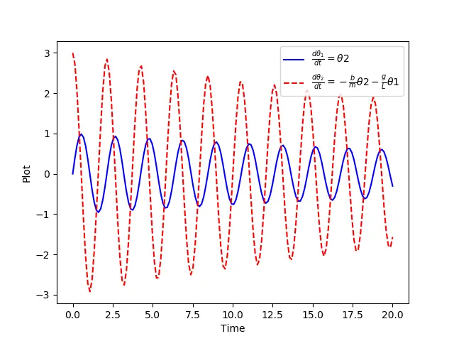
• Now we need to plot the displacement and velocity wrt time. The plots obtained can be seen as damped at the end of time interval due to damping coefficient.

Results:

• In the below figure we can observe the displacement – velocity is plotted as below:

• The animation of pendulum can be seen in the below link:

  https://youtu.be/OjLVQoa9sZo

  Conclusion: As discussed a plot of displacement- velocity wrt is studied and projected. The animation required for showing the projectile of pendulum is constructed.