Week 3 - Solving second order ODEs

OBJECTIVE

• To write a program in python to simulate the transient behavior of a Simple pendulum.
• To plot graph Time vs Displacement.
• To create an animation of its motion.

THEORY :

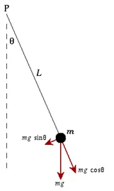
A pendulum is a simple mechanical system that obeys differential equations. The pendulum is initially at rest vertically. If you move the pendulum by an angle θ and let go, gravity will cause the pendulum to return to its original position.

A pendulum is a weight suspended from a pivot so that it swings freely. When the pendulum is laterally displaced from its equilibrium rest position, it experiences the restoring force of gravity and accelerates back to its equilibrium position. When released, the restoring force on the pendulum mass causes the pendulum to oscillate about its equilibrium position and oscillate back and forth. The time of one complete cycle, i.e. one left swing and one right swing, is called duration. The period depends on the length of the pendulum and somewhat on the amplitude, or width of the swing.

GOVERNING EQUATION

Second order differential equation for simple pendulum is

d2θdt2+bmdθdt+glsinθ=0d2θdt2+bmdθdt+glsinθ=0

Where,

g=gravity (ms2ms2)

l=Length of the pendulum (m)

m=mass of the ball (kg)

b=damping coefficient

INPUT VALUES

g=9.81 ms2ms2

l=1 m

b=0.05 m

m=1 kg

PROCEDURE:

• First, import the 'matplotlib.pyplot', 'math', 'scipy' and 'numpy' libraries for computation.
• The Scipy library provides a second-order ODE equation for solving theta.
• Then we can calculate the other parameters just by entering the given parameters g, b, l, m.
• Call a theta value in a function call instruction and specify the step in time using the numpy command.
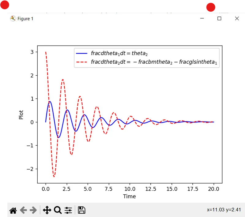
• Next, plot a displacement plot against time.
• For simple pendulum motion, first enter the pendulum start (x0, y0) and end (x1, y1) coordinates.
• String and Counter commands save all PNG files with different PNG names.
• For the animation, we use another software to create the animation.

PROGRAM:

Python 3.10.7 (tags/v3.10.7:6cc6b13, Sep  5 2022, 14:08:36) [MSC v.1933 64 bit (AMD64)] on win32
Type "help", "copyright", "credits" or "license()" for more information.
import math
import matplotlib.pyplot as plt
import numpy as np
from scipy.integrate import odeint

def model(theta,time,b,g,l,m):
	theta1 = theta[0]
	theta2 = theta[1]
	dtheta1_dt = theta2
	dtheta2_dt = -(b/m)*theta2 - (g/l)*math.sin(theta1)
	dtheta_dt = [dtheta1_dt,dtheta2_dt]
	return dtheta_dt

b = 0.05
g = 9.81
l = 1
m = 0.1

# initial condition
theta_0 = [0,3]

# time points
time = np.linspace(0,20,300)
... 
... # Solving ODE
... theta = odeint(model,theta_0,time,args = (b,g,l,m))
... 
... 
... Angular_displacement = []
... Angular_velocity = []
... 
... for j in range(0,len(theta)):
... 	displacement = theta[j,0]
... 	Angular_displacement.append(displacement)
... 
... 	velocity = theta[j,1]
... 	Angular_velocity.append(velocity)
... 
... 
... 
... #Creating a for loop to make arrays of angular displacement and velocity
... 
... 
... # plotting the results
... 
... plt.figure(1)
... plt.plot(time,theta[:,0],'b-',label = r'$frac{dtheta_1}{dt} = theta_2$')
... plt.plot(time,theta[:,1],'r--',label = r'$frac{dtheta_2}{dt} = -frac{b}{m}theta_2 - frac{g}{l}sintheta_1$')
... plt.xlabel('Time')
... plt.ylabel('Plot')
... plt.legend(loc = 'best')
... plt.show()
... 
... # Simulating the simple pendulum
... x0 = 0
... y0 = 0
... # creating a for loop to simulate the simple pendulum
... ct = 1
... for i in range(0,len(time)):
... 	THETA = Angular_displacement[i]
... 	x1 = l*math.sin(THETA)
... 	y1 = -l*math.cos(THETA)
... 	filename = 'pendulum%05d' % ct
... 	ct = ct + 1
... 
... 
... 	plt.figure(2)
... 	plt.plot([-1,1],[0,0],color = 'r')
... 	plt.plot([x0,x1],[y0,y1])
... 	plt.plot(x1,y1,marker = 'o',markerfacecolor = 'g',markeredgecolor  = 'k',markersize = 15)
	plt.xlim([-2,3])
	plt.ylim([-3,3])
	plt.title('Animation of Simple pendulum motion',fontsize = 20,fontweight = 'bold')
	plt.savefig(filename)

RESULTS

Plot

Animation (Gif)

CONCLUSION

• Simulation of transient behavior of a Simple pendulum motion by solving second order differential equation.
• Animation of the Simple pendulum is simulated.