Project 2 - Rankine cycle Simulator

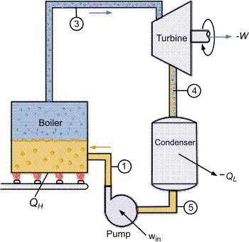
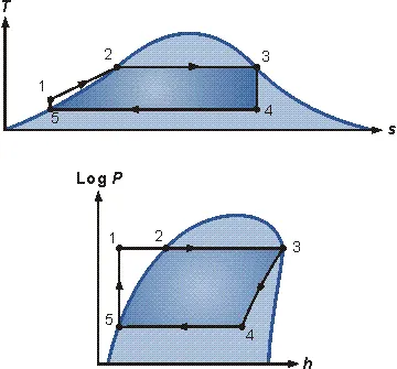
The Rankine cycle is the fundamental operating cycle of all power plants where an operating fluid is continuously evaporated and condensed. The selection of operating fluid depends mainly on the available temperature range. FIG2 shows the idealized Rankine cycle.

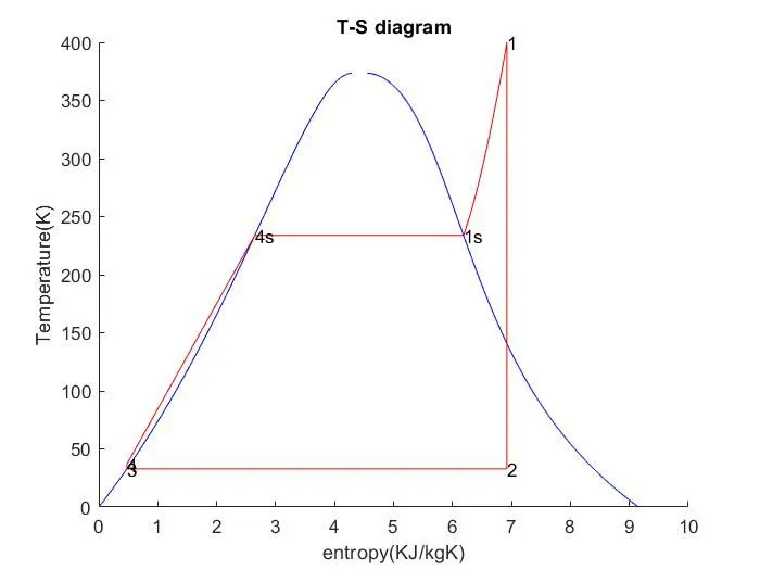
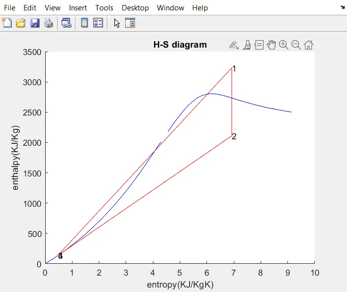
The pressure-enthalpy (p-h) and temperature-entropy (T-s) diagrams of this cycle are given in FIG2. The Rankine cycle operates in the following steps:

• 1-2-3 Isobaric Heat Transfer. High pressure liquid enters the boiler from the feed pump (1) and is heated to the saturation temperature (2). Further addition of energy causes evaporation of the liquid until it is fully converted to saturated steam (3).
• 3-4 Isentropic Expansion. The vapor is expanded in the turbine, thus producing work which may be converted to electricity. In practice, the expansion is limited by the temperature of the cooling medium and by the erosion of the turbine blades by liquid entrainment in the vapor stream as the process moves further into the two-phase region. Exit vapor qualities should be greater than 90%.
• 4-5 Isobaric Heat Rejection. The vapor-liquid mixture leaving the turbine (4) is condensed at low pressure, usually in a surface condenser using cooling water. In well designed and maintained condensers, the pressure of the vapor is well below atmospheric pressure, approaching the saturation pressure of the operating fluid at the cooling water temperature.
• 5-1 Isentropic Compression. The pressure of the condensate is raised in the feed pump. Because of the low specific volume of liquids, the pump work is relatively small and often neglected in thermodynamic calculations.

CODE

clear all
close all
clc

disp('RANKINE CYCLE SIMULATOR');
disp('1-2 = isentropic expansion in the turbine');
disp('2-3 = constant pressure heat rejection by the condensor');
disp('3-4 = isentropic compression in the pump');
disp('4-1 = constant pressure heat addition by the boiler');

%To GIVE the inputs and getting the text as given in the problem

t1 = input('enter the temperature at the turbine inlet (in degree celsius):');

p1=input('enter the pressure at the turbine inlet (in bar):');
p2=input('enter the pressure at the condensor (in bar)');

fprintf('rRESULTSrn')

%stage 1 (turbine inlet)
s1= XSteam('s_pT',p1,t1);
h1=XSteam('h_pT',p1,t1);

%stage 2 condenser inlet
sf2 = XSteam('sL_p',p2);
sg2 = XSteam('sV_p',p2);
hf2 = XSteam('hL_p',p2);
hg2 = XSteam('hV_p',p2);

s2 = s1;
t2 = XSteam('Tsat_p',p2);

%splitting the formulae

x2=((s2-sf2)/(sg2-sf2));
h2=hf2+(x2*(hg2-hf2));

%stage3 (pump inlet)
p3=p2;
t3=XSteam('Tsat_p',p2);
s3=XSteam('sL_p',p3);
h3=XSteam('hL_p',p3);

cp4 = XSteam('cpL_p',p3);
cv4 = XSteam('cvL_p',p3);
gamma = (cp4/cv4);
g = (gamma-1)/gamma;

%stage 4(boiler inlet)

p4=p1;
s4=s3;
h4 = XSteam('h_ps',p4,s4);
t4=t3*((p4/p3)^g);

%turbine work
wt=h1-h2;
%pump work
wp=h4-h3;
%network
w_net=wt-wp;

%Heat in and out of the system
q_in=h1-h4;
q_out=h2-h3;

q_in=h1-h4;
q_out=h2-h3;

n=w_net/q_in;
np=n*100;

SSC=3600/w_net;
tf_sat=XSteam('Tsat_p',p1);
sf_sat=XSteam('sL_p',p1);
hf_sat=XSteam('hL_p',p1);
sg_sat=XSteam('sV_p',p1);
hg_sat=XSteam('hV_p',p1);

%plot figure 1
figure(1)
hold on
temp=linspace(0,400,1000);
for i=1:length(temp)
aa(i) =XSteam('sL_T',temp(i));

end

for j=1:length(temp)
bb(j)=XSteam('sV_T',temp(j));
end

plot(aa,temp,'color','b')
plot(bb,temp,'color','b')

temp=(XSteam('Tsat_p',p1));
t0=linspace(temp,t1,300);
for i=1:length(t0)
c11(i)=XSteam('s_pt',p1,t0(i));
end

t5=XSteam('Tsat_p',p4);
s5=XSteam('sL_T',t5);

plot([s1 s2],[t1 t2],'color','r')
plot([s2 s3],[t2 t3],'color','r')
plot([s3 s4],[t3 t4],'color','r')
plot([s4 s5],[t4 t5],'color','r')
plot([sf_sat sg_sat],[tf_sat tf_sat],'color','r')
plot(c11,t0,'color','r')

title('T-S diagram')
xlabel('entropy(KJ/kgK)')
ylabel('Temperature(K)')

text(s1,t1,'1');
text(s2,t2,'2');
text(s3,t3,'3');
text(s4,t4,'4');
text(s5,t5,'4s');
text(sg_sat,tf_sat,'1s');

%plotting figure 2
figure(2)
hold on

temp1=linspace(0,400,1000);
for i=1:length(temp1)
cc(i)=XSteam('hL_T',temp1(i));
end

for j=1:length(temp1)
dd(j)=XSteam('hV_T',temp1(j));

end

plot(aa,cc,'color','b')
plot(bb,dd,'color','b')

plot([s1 s2],[h1 h2],'color','r')
plot([s2 s3],[h2 h3],'color','r')
plot([s3 s4],[h3 h4],'color','r')
plot([s4 s1],[h4 h1],'color','r')

title('H-S diagram')
xlabel('entropy(KJ/KgK)')
ylabel('enthalpy(KJ/Kg)')

text(s1,h1,'1');
text(s2,h2,'2');
text(s3,h3,'3');
text(s4,h4,'4');

%printing the output

fprintf('at stage point 1:n')
fprintf('P1 is : %f barn',p1)
fprintf('T1 is : %f deg celsiusn',p1)
fprintf('T1 is :%f KJ/kgn',h1)
fprintf('S1 is: %f KJ/KgKrn',s1)

disp('at state point 2:')
fprintf('P2 is : %f Barn',p2)
fprintf('T2 is : %f deg celsiusn',t2)
fprintf('H2 is : %f KJ/Kgn',h2)
fprintf('S2 is : %f KJ/KgKn',s2)
fprintf('X is : %f rn',x2)

disp('at state point 3:')
fprintf('P3 is : %f Barn',p3)
fprintf('T3 is : %f deg celsius400n',t3)
fprintf('H3 is : %f KJ/Kgn',h3)
fprintf('S2 is : %f KJ/KgKbn',s3)

disp('at state point 4:')
fprintf('P4 is : %f Barn',p4)
fprintf('T4 is : %f deg celsiusn',t4)
fprintf('H4 is : %f KJ/Kgn',h4)
fprintf('S4 is : %f KJ/KgKbn',s4)

fprintf('Wt : %f KJ/Kgn',wt)
fprintf('Wp : %f KJ/Kgn',wp)
fprintf('Wnet : %f KJ/Kgn',w_net)
fprintf('Ntherm : %f %%n',n*100)
fprintf('SSC : %f KJ/KWhbn',SSC)

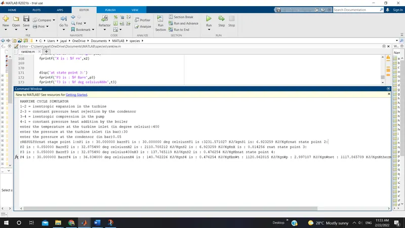
RESULTS: