Week 3 - Solving second order ODEs

SOLVING SECOND ORDER ODEs

To write a program that solves the following ODE. ODE represents the equation of motion of a simple pendulum with damping

i.e., A program that simulates the pendulum motion

`(d^2theta)/dt + (b/m)((d theta)/dt) + (g/l) sin theta = 0`

L=1 metre,

m=1 kg,

b=0.05.

g=9.81 m/s2.

Simulate the motion between 0-20 sec, for angular displacement=0,angular velocity=3 rad/sec at time t=0.

APPROACHES MADE:

------> Discretisation of ODE

------> Initialisation of variables/Inpuuts

------> Solving ODE using solver ODEint

------> Making a pendulum animation

ODEINT is a ordinary differential equation integration library which is a collection of advanced numerical algorithms to solve initial-value problems of ordinary differential equations.Here odeint command is used to solve the 2 first order ODE equation and results have been plotted.

PROGRAM:

import math
import numpy as np
import matplotlib.pyplot as plt
from scipy.integrate import odeint

def model (initial,t,b,l,g,m):
 t1=initial[0]
 t2=initial[1]
 dt1=t2
 dt2=(-b*t2/m)-(g*math.sin(t1)/1)
 dt=[dt1,dt2]
 return dt

b=0.05
g=9.8
l=1
m=1

initial =[0,3]
time=np.linspace(0,20,200)
dis_v=odeint(model,initial,time,args=(b,l,g,m))

plt.plot(time,dis_v[:,0],'--',label='displacement')

plt.plot(time,dis_v[:,1],'-',label='velocity')
plt.legend()
plt.xlabel('time')
plt.ylabel('displacement velocity')
plt.title('Time vs Displacement velocity')
plt.show()

y=dis_v[:,0]
ct=1
for theta in y:
	x1=0;y1=0
	x2=l*math.sin(theta)
	y2=l*math.cos(theta)
file='test%05d.png'%ct
plt.figure()
plt.plot([-1.5,1.5],[0,0],linewidth=8)
plt.plot([x1,x2],[y1,y2],linewidth=3)
plt.plot(x2,y2,'o',markersize=15)
plt.xlim([-1.5,1.5])
plt.ylim([-1.5,1.5])
plt.savefig(file)
ct=ct+1

PLOT OBTAINED:

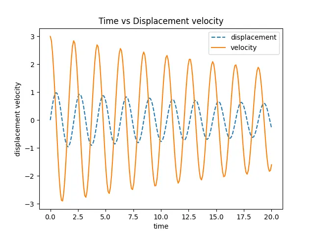
ANIMATION :
https://youtu.be/LxARGaqrbng