Week 3 - Solving second order ODEs

Aim: The aim of this challenge is to solve second order ODEs using Python.

Objectives: The objectives of this challenge is to

• Identifying the governing ordinary differential equations for a pendulum
• Solving the ODEs using Python
• Plotting the displacement and velocity profiles
• Simulate the damping effect on the pendulum by creating an animation

ODE representing the motion of pendulum:

In the above equation,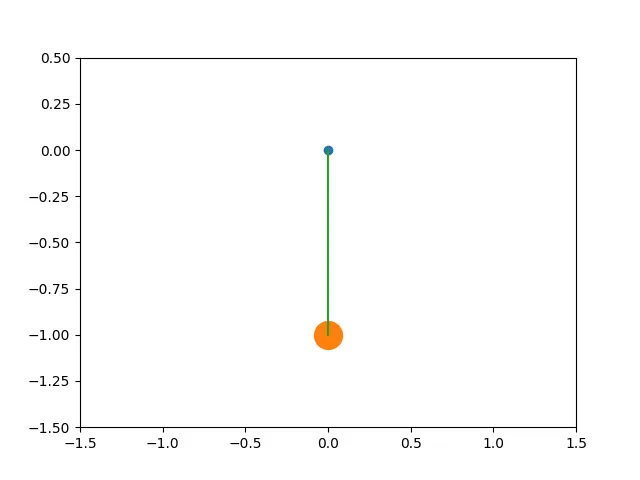

g = gravity in m/s2,

L = length of the pendulum in m,

m = mass of the ball in kg,

b=damping coefficient.

Since the ODE is of order 2, it is broken down into two equations of the first-order ODE.

Let displacement θ=θ1

dθdt=dθ1dt=θ2dθdt=dθ1dt=θ2

dθ2dt=−(b/m)θ2−(g/l)sinθ1

#Python code to solver pendulum ODE
import math
from scipy.integrate import odeint
import numpy as np
import matplotlib.pyplot as plt

#Defining function
def model(theta,t,b,g,l,m):

theta1 = theta[0] # Intial Condition for First FODE
theta2 = theta[1] # Initial condition for Second FODE

dtheta_1 = theta2 # First FODE
dtheta_2 = -(b/m)*theta2-(g/l)*math.sin(theta1) # Second FODE
dtheta = [dtheta_1,dtheta_2]
return dtheta

b = 0.05
l = 1
g = 9.81
m = 1

#Initial Condition
theta_in = [0, 3]

#Time points
t = np.linspace(0,20,250)

#ODE Solver
theta = odeint(model,theta_in,t,args = (b,g,l,m))

#Angular velocity and displacement plot wrt time
plt.figure(1)
plt.plot(t,theta[:,0],'b-',label=r'$frac{d theta1}{dt}= theta2$')
plt.plot(t,theta[:,1],'r-',label=r'$frac{d theta2}{dt}= -(b/m)*theta2-(g/l)*sin(theta1)$')
plt.xlabel('Time')
plt.ylabel('Plot')
plt.title('Pendulum displacement and velocity plot')
plt.legend()
plt.savefig('Pendulum displacement and velocity plot')
plt.show()

#Base points for pendulum
x_0 = 0
y_0 = 0

ct = 0

#Pendulum animation
angle = theta[:,0]
for value in angle:
filename = str(ct) + '.png' #
ct = ct+1
plt.figure()
x1 = l*math.sin(value)
y1 = -l*math.cos(value)
plt.xlim([-1.5,1.5])
plt.ylim([-1.5,0.5])
plt.plot(x_0,y_0,marker='o')
plt.plot(x1,y1,marker = 'o', ms = 20)
plt.plot([x_0,x1],[y_0,y1])
plt.savefig(filename)

Result:

Plot:
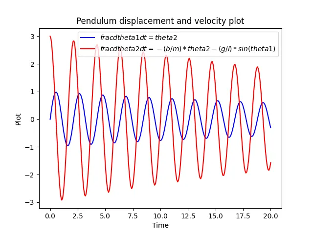
The Red line shows the displacement plot and the blue line the angular velocity plot. The damping effect is not clearly visible because the system has a low damping coefficient.

GIF:

The bob is initially at resting position and an angular velocity of 3rad/s is applied to it.