Week 3 - Solving second order ODEs

Aim: To create a program to describe the transient behavior of a simple pendulum and to simulate the animation of the motion of pendulum w.r.t the data given

Points to remember: it's important to start with clear all, close all and clc commands

Clear all - removes data from the workspace, freeing up system memory

Close all- deletes the current figure or the specified figure

clc - clears all input and output from the Command Window display, giving you a clean screen

Programming :

* The ODE45 integrate the function using numerical integration technique Runge Kutta Method.

* The ODE45 is an integrated command in Matlab which solves ordinary differential equation.

* Specify the inputs to the matlab as given in the question.

* Define the initial condition as angular displacement and angular velocity have been defined from the question Timespan has also defined.

* Create a function for ode45 for calling the function while coding the main script the input to the function has been integrated throught inputs.

* [t,results] time and initial condition will be calculated via given input and ODE45 command and function calling.

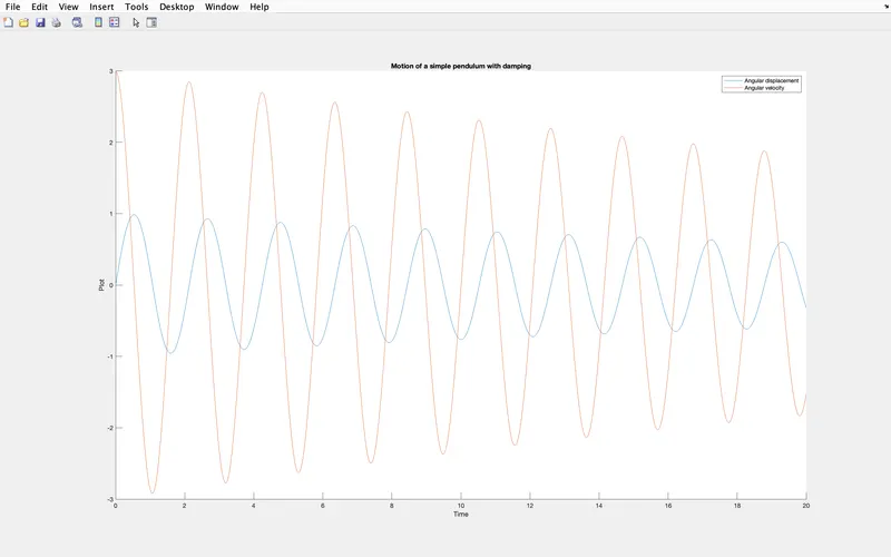
* The output is then plotted (angular displacement w.r.t time , angular velocity w.r.t time)

function [dtheta_dt]= ode_solver(t,theta,b,g,l,m)

theta1 = theta(1)
theta2 = theta(2)
dtheta1_dt = theta2;
dtheta2_dt = -(b/m)*theta2 - (g/l)*sin(theta1);
dtheta_dt = [dtheta1_dt;dtheta2_dt];

end

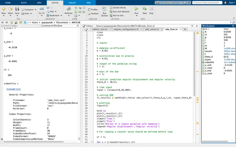
clear
close
clc

% inputs

% damping co-efficient 
b = 0.05;

% acceleration due to gravity 
g = 9.81;

% length of the pendulum string 
l = 1;

% mass of the bob 
m = 1;

% initial condition angular displacement and angular velocity 
theta_0 = [0;3];

% time input 
tspan = linspace(0,20,500);

% solving ODE 
[t,results] = ode45(@(t,theta) ode_solver(t,theta,b,g,l,m), tspan,theta_0)

% plotting
figure(1)

hold on
plot(t,results(:,1))
plot(t,results(:,2))
xlabel('Time')
ylabel('Plot')
title('Motion of a simple pendulum with damping')
legend('Angular displacement','Angular velocity')

% For looping a counter value should be defined before loop

ct = 1;

for i = 1:length(results(:,1))
    x_start = 0
    y_start = 0
    x_end = l*sin(results(i,1))
    y_end = -l*cos(results(i,1))

    % plotting for animation
    figure(2)
    plot([-1 1],[0 0],'LineWidth',3)
    hold on
    plot([x_start x_end],[y_start y_end],'LineWidth',3)
    hold on
    
    plot(x_end,y_end,'o','markersize',20,'MarkerFaceColor','y')
    title('Animation of the behaviour of a pendulum')
    axis([-1.5 1.5 -1.5 1])
    pause(0.03)
    hold off
    M(ct)=getframe(gcf);
    ct=ct+1
end

 % movie of the pendulum


movie(M)
videofile=VideoWriter('ode_func.avi','uncompressed avi')
open(videofile)
writeVideo(videofile,M)
close(videofile)

The youtube link for the animation, Motion of pendulum

https://youtu.be/VKmsTwQmz6A