Week 3 - Solving second order ODEs

THEORY:-Ordinary Differential Equations(ODEs), An odinary differential equation containing one or more functions of one indipendent variable and the derivatives of those functions.

-The term ordinary is in contrast with the term partial differential equation which may be w.r.t more then one independent variable.

Simple pendulum:-

In Engineering, ODE is used to describe the transient behavior of a system. A simple example is a pendulum

The way the pendulum moves depends on the Newtons second law. When this law is written down, we get a second order Ordinary Differential Equation that describes the position of the "ball" w.r.t time.

Similarly, there are hundreds of ODEs that describe key phenomena and if you have the ability to solve these equations then you will be able to simulate any of theses systems.

Your objective is to write a program that solves the following ODE. This ODE represents the equation of motion of a simple pendulum with damping

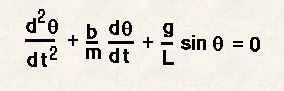
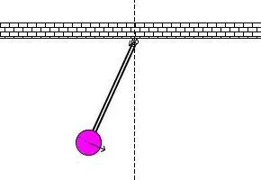
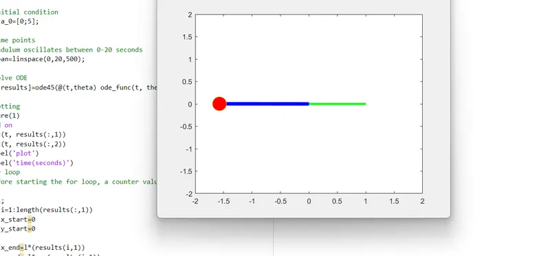
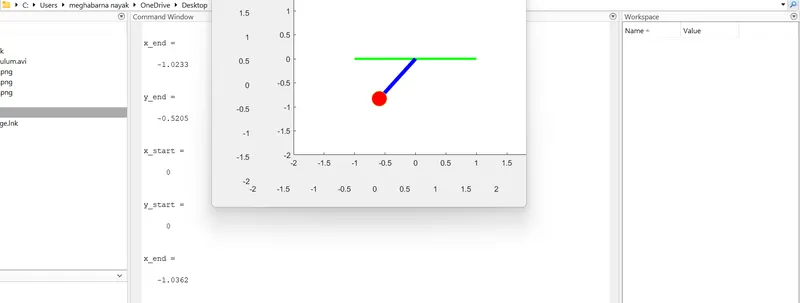
In the above equation, g = gravity in m/s2, L = length of the pendulum in m, m = mass of the ball in kg, b=damping coefficient. Write a program in Matlab\Octave that will simulate the pendulum motion, just like the one shown in the start of this challenge. use, L=1 metre, m=1 kg, b=0.05. g=9.81 m/s2. Simulate the motion between 0-20 sec, for angular displacement=0,angular velocity=3 rad/sec at time t=0. When you do this you will get the position of the pendulum as a function of time. Use this information to animate the motion of the pendulum, as shown in the below figure.

MATLAB CODE:-

lear all
close all
clc

b=0.05;
g=9.81;
l=1;
m=1;

% initial condition
theta_0=[0;5];

% time points
%pendulum oscillates between 0-20 seconds
t_span=linspace(0,20,500);

% solve ODE
[t, results]=ode45(@(t,theta) ode_func(t, theta, b,g,l,m),t_span, theta_0);

%plotting
figure(1)
hold on
plot(t, results(:,1))
plot(t, results(:,2))
xlabel('plot')
ylabel('time(seconds)') 
%for loop
%Before starting the for loop, a counter value was defined

ct=1;
for i=1:length(results(:,1))
    x_start=0
    y_start=0
    
    x_end=l*sin(results(i,1))
    y_end=-l*cos(results(i,1))

    %ploting the animation
    figure(2)

    plot([-1 1], [0 0],'LineWidth',3,'color','green')
    hold on


    %starting of pendulum 
    plot([x_start, x_end],[y_start y_end],'LineWidth',5,'color','b')
    hold on
    %Bob of pendulum,
    plot(x_end,y_end,'o','Markersize',20,'MarkerFaceColor','r')
    axis([-2 2 -2 2])
    pause(0.01)
    

    M(ct)=getframe(gcf);
    ct=ct+1;
    hold off
end   

% Animation of the pendulum

movie(M)
videofile=VideoWriter('simple_pendulum.avi','Uncompressed AVI');
open(videofile)
writeVideo(videofile,M)
close(videofile)

OUTPUT:-

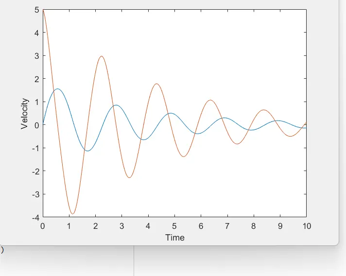
The output obtained is graphical representation of velocity curve w.r.t time.

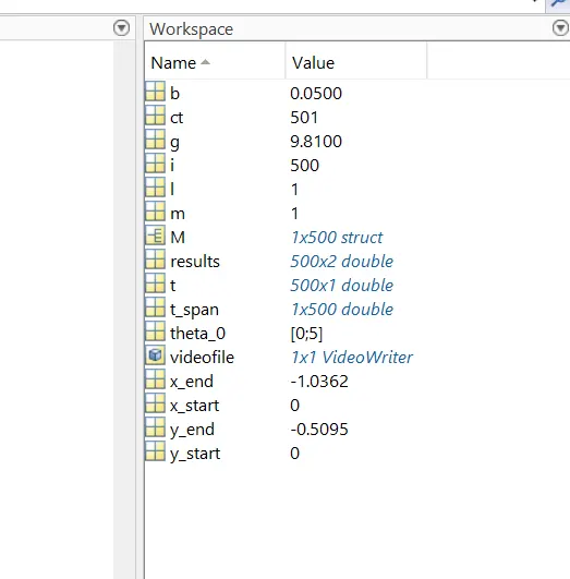
WORKSPACE:-

CONCLUSION;-

Analyse and understood the equation of motion with damping of a simple pendulum and create a programe for solving ode for pendulum ode45 equation solver for the transient behaviuour of the system and animate the motipon of the pendulum when the displacement changes with respect to time