Week 3 - Solving second order ODEs

Newton's second low is given by:

F = m*a

where:

F is force in N

m is the mass of the object in kg

a is the acceleration due to gravity in m/s^2

Ordinery Differential Equation-ODE

Differential equation is used to relates the one or more functions and its derivatives.

here we going to relate the two functions lsuch as time and angular displacement.

t and theta are the function here.

Here pednulum acts like a spring, When apply the force on the pendulum ball will create the to and fro angular motion.

one end of the pendulum is fixed and another end is free to rotate.

ODE here used to study the movement of pendulum.

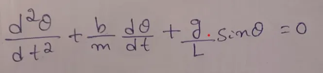
d^2theta/dt^2 + b/m*dtheta/dt + g/L*sintheta = 0

Where:

g = Acceleration due to gravity in m/s2

L = length of the pendulum in m

m = mass of the ball attached to the pedulum rod in kg

b=damping coefficient

Given set of data:

L=1 metre

m=1 kg

b=0.05

g=9.81 m/s2

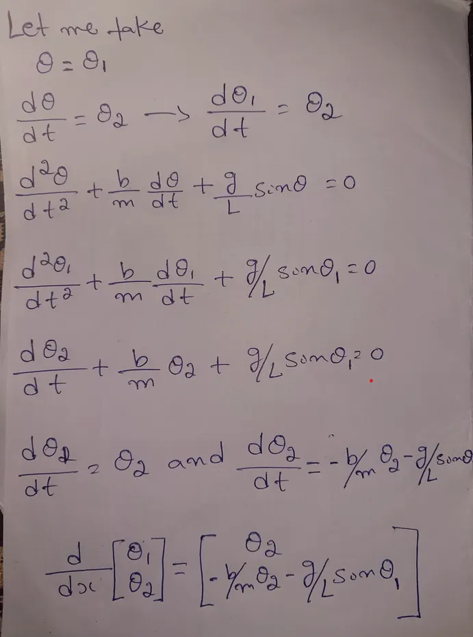
First need to brake the second order ODE into two first order ODEs

let me take

theta = theta1

dtheta/dt = theta2

so

dtheta1/dt = theta2

Second order ODE is given below

d^2theta/dt^2 + b/m*dtheta/dt + g/L*sintheta = 0

Put the theta1 in the above equation

Equation becomes like below

d^theta1/dt^2 + b/m*dthet1/dt + g/L*sintheta1 = 0

Put the theta2 in the above equation

Equation becomes like below

dtheta2/dt + b/m*theta2 + g/L*sintheta1 = 0

dtheta1/dt = theta2 is the first order ode - Number 1

dtheta2/dt = -b/mtheta2-g/L*sintheta1 - number 2

Derivation breakup image

Here is the function script:

Function file name is ode_function

Inputs to ode_function are t,theta,b,g,l and m.

function [dtheta_dt] = ode_function(t,theta,b,g,l,m)
theta1 = theta(1)
theta2 = theta(2)
dtheta1_dt = theta2;
dtheta2_dt = -(b/m)*theta2-(g/l)*sin(theta1);
dtheta_dt = [dtheta1_dt; dtheta2_dt];

Put the two first order OED in the form of column vector shown above.

Here is the main simulation script:

% Inputs are as follows

% Damping coefficient

b = 0.05;

% Acceleraton due to gravity in m/s^2

g = 9.81;

% Mass of the bob in kg

m = 1;

%Length of the pendulum rod in metres

l = 1;

% Initial condition

dis_angvelo = [0;3];

% Timerange

t_span = linspace(0,20,500);

% Solving ode

[a,b] = ode45(@(t,theta) ode_function(t,theta,b,g,l,m),t_span,dis_angvelo);

% Plotting

figure(1)

plot(a,b(:,1),'linewidth',1)

hold on

plot(a,b(:,2),'linewidth',1)

axis([0 25 -3 3])

xlabel('Time - sec')

ylabel('Angular Velocity & Displacement')

legend('change in displacement','change in angular velocity')

hold off

figure(2)

plot(b(:,1),b(:,2))

xlabel('Position - rad')

ylabel('Angular Velocity - rad/sec')

Simulation creation program:

theta2 = b(:,1);

ct = 1;

for i = 1:length(theta2);

theta3 = theta2(i);

x0 = 0;

y0 = 0;

x1 = l*sin(theta3);

y1 = -l*cos(theta3);

figure(3)

plot([x0 x1],[y0 y1],'color','r','linewidth',2)

hold on

plot(x1,y1,'o','markers',10,'markerfacecolor','b')

hold off

grid on

axis([-1.5 1.5 -1.5 0.5])

pause(0.003)

M(ct) = getframe(gcf);

ct = ct+1;

end

% movie making scropt

movie(M)

videofile = VideoWriter('pendulum.avi','uncompressed avi');

open(videofile)

writeVideo(videofile,M)

close(videofile)

Outpts and results are given below

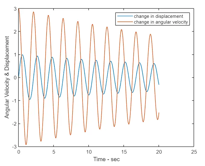
This plot shows the how angular velocity and angular displacement changes with respect to time changes.

Here angular velocity starts from 3 radians/sec and angular displacement is starts from 0 radians.

Time starts from 0 to 20 sec range, We can see the angular velocity and angular displacement values.

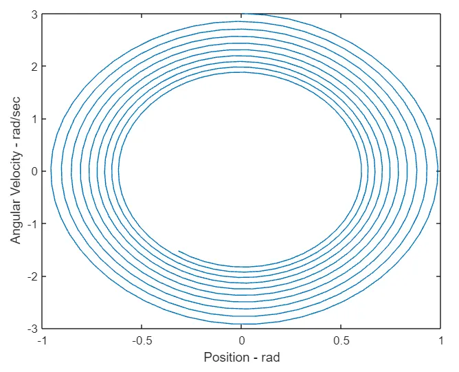
Here we can analysis the angular displacement in radians versus angular velocity in radians/sec

Kindly find the attached vedio of the pendulum movement.

Thanks,

Siddesh R S